Report of
RV Ronald H. Brown Cruise 06-03
to the
Western Subtropical and Tropical North Atlantic
10 April to 30 April, 2006
This report was prepared by Peter Wiebe, Larry Madin, Francesc Pagès, Dhugal Lindsay, Hege Øverbø Hansen, Saramma Panampunnayil, Martin Angel, Hiroyuki Matsuura, Mikiko Kuriyama, Astrid Cornils, Russ Hopcroft, Colomban de Vargas, Silvia Watanabe, Yurika Ujiie, Hui Liu, Barbara Costas, Tracey Sutton, C. B. Lalithambika Devi, Rob Jennings, Paola Batta Lona, Brian Ortman, Ebru Unal, Leo Blanco Bercial, Nancy Copley, Chaolun Li, Joe Catron, and Dicky Allison.
A
Census of Marine Zooplankton (CMarZ)
Report
Available online from the
CMarZ website,
www.cmarz.org

Acknowledgments
This was the first major CMarZ cruise in the Western North Atlantic. The success of the cruise was due to the collective efforts of Captain, Officers, Crew, and all members of the Scientific Party. Throughout the cruise there was a camaraderie and friendliness among all the participants that made this expedition a great pleasure. This cruise was supported by the NOAA Ocean Exploration Program.

RB06-03 CMarZ Cruise Participants on the RV R.H. Brown
Sitting Row 1 (L-R):Chaolun Li, Saramma Panampunnayil, Silvia Watanabe, Hui Liu, Francesc Pagès, Paola Batta Lona, Tracey Sutton, Martin Angel, Dicky Allison.
Standing Row 1 (L-R): Mikiko Kuriyama, Lalithambika Devi, Brian Ortman, Russ Hopcroft, Nancy Copley, Ebru Unal, Joe Catron.
Standing Row 2 (L-R): Yurika Ujiie, Leo Blanco Bercial, Hiroyuki Matsuura, Larry Madin, Barbara Costas, Hege Øverbø Hansen.
Back Row 3: Colomban de Vargas, Astrid Cornils, Erich Horgan, Dhugal Lindsay, Rob Jennings, Peter Wiebe.
TABLE OF CONTENTS
MOCNESS and OTHER SAMPLING, and SAMPLE PROTOCOLS
2.0 Blue-water SCUBA diving for gelatinous zooplankton.
5.0 Sample Processing Protocol.
WATER COLUMN STRUCTURE AT THE STATIONS
4.0 Ctenophores, Amphipods, and Cephalopods
9.0 Calanoid copepods in the genus Euaugaptilus and the family Scolecitrichidae
10.0 Calanoid copepods primarily Aetideidae and Heterorhabdidae
11.0 Other Copepods Identified on RHB06-03.
12.0 Larvaceans and Planktonic Molluscs
13.0 Skeletonized Microplankton
14.0 Microzooplankton – Tintinnids
14.3 Discussion/Preliminary Observation
18.0 Silhouette photography, CMarz web site
18.1 Silhouette Photography (N. Copley)
19.0 Training on Zooplankton Sampling and Molecular Analysis
20.0 ARMADA Teacher at Sea Project
APPENDIX 2. Summary of Blue Water Dive Collections
APPENDIX 3. List of DNA extractions from foraminifera.
APPENDIX 4. Colonial radiolarians collected by diving
APPENDIX 5. Tintinnid images and designations followed by preliminary ID
APPENDIX 6. MOCNESS Deployment Log.
The focus of the CMarZ program is on the development of a taxonomically comprehensive assessment of biodiversity of animal plankton throughout the world ocean. The project goal is to produce accurate and complete information on zooplankton species diversity, biomass, biogeographical distribution, genetic diversity, and community structure by 2010. Our taxonomic focus is the animals that drift with ocean currents throughout their lives (i.e., the holozooplankton). This assemblage currently includes ~6,800 described species in fifteen phyla; our expectation is that at least that many new species will be discovered as a result of our efforts. The Census of Marine Zooplankton (CMarZ) program is an ocean realm field project of the Census of Marine Life (CoML).
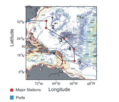 Figure 1. Trackline and station positions on
CMarZ Cruise
RB06-03, 10 to 30 April 2006. The cruise started in
Charleston, SC and ended in San Juan, Puerto Rico.
Figure 1. Trackline and station positions on
CMarZ Cruise
RB06-03, 10 to 30 April 2006. The cruise started in
Charleston, SC and ended in San Juan, Puerto Rico.On this cruise, the focus was the tropical/subtropical waters of the Atlantic Ocean west of the mid-Atlantic ridge. The objective was to collect and identify the zooplankton distributed throughout the entire water column, with a particular focus on the under-sampled mesopelagic, bathypelagic, abyssopelagic zones, and then to sequence them genetically at sea. Thus, the scientific participants on this cruise include CMarZ researchers, expert taxonomists, molecular specialists, staff, and students. Sampling was conducted along a transect extending from the northern Sargasso Sea to the equatorial waters northeast of Brazil (Figure 1). At five primary stations, environmental data and zooplankton samples were collected using three Multiple Opening/Closing Nets and Environmental Sensing Systems (MOCNESS). One was a large opening/closing trawl and two were smaller multiple net systems (See MOCNESS Sampling section below for more detail). Other samples were collected with ring nets and water bottles, and by blue water SCUBA diving.
Samples were analyzed at sea using traditional taxonomic approaches and molecular systematic analysis, including DNA sequencing of a target gene portion for each species. After the cruise, follow-up molecular analysis, species counts, and expert taxonomic evaluation and description of any putative new or undescribed species will be done in association with the CMarZ Taxonomic Network. In addition to the intensive sampling of the water column, a series of lectures and workshops were conducted as part of the at-sea training in zooplankton morphological and molecular systematic approaches.
10 to 12 April 2006: The cruise got underway at 1400 on 10 April when we left the port of Charleston, South Carolina after four days of intense set-up of the equipment and laboratory spaces needed for the work at sea. Shortly after leaving the dock, the ship spent time in Charleston Harbor while a calibration of the Robertson Navigation system took place, which had undergone repairs while the ship was in port.
The R/V Ron Brown finally left the harbor and got underway for the first station located in the Northern Sargasso Sea about 1800. During the early hours of the night of the 10th, the ship’s ride was comfortable, but the winds picked up to around 20 kts towards the morning of the 11th as we steamed out across the continental shelf and the Gulf Stream, and the motion of the vessel made many of the scientific party a bit seasick. The moderately rough weather continued into daylight on the 11th of April and the loading of nets onto the three Multiple Opening/Closing Nets and Environmental Sensing Systems (MOCNESS) and other work in the laboratories went slowly. The initial abandon ship and the fire and boat drill took place around 1030.
Problems with the operation of the trawl winch with 0.68" conducting cable, which was the mainstay of our sampling program, had been identified a couple of weeks before the start of the cruise and most of the repairs had taken place by the time the ship left the dock. On the evening of the 11th, 8000 meters of trawl wire was streamed to test the ability of the winch to carry out the deep MOCNESS tows. Although the winch had no difficulty in paying the cable out, there was significant difficulty bringing the wire back on board at a reasonable haul in speed. During the test, a load cell burnt out and it was replaced. A second test took place on the evening of the 12th. This test indicated that the winch could be used to tow the MOCNESS trawl to bathy- and abyssopelagic depths.
Several science meetings took place during the steaming to Station 1. On the evening of the 11th, there was an introductory meeting to discuss the cruise objectives and to review plans for work at the stations. On the afternoon of the 12th there were two additional meetings. The first was to work out the final details of the sampling at a station and the protocols for how each of the zooplankton samples was to be processed. The second involved a number of the officers and crew and was focused on the methods of deployment of the over-the-side equipment and who would be in charge of coordinating them.
During the afternoon of the 11th, a ½-m diameter ring net was deployed to 100 m to provide a collection of zooplankton that could be used by the taxonomic experts on board to begin their work on this cruise. A number of species of copepods, ostracods, gelatinous animals, formaminifera, and other groups were picked live from the sample and a number of the species were identified. Some of these were then selected for genetic sequencing on the 12th. Earlier in this day, a first occurred when a zooplankton species (a copepod, Disseta grandis, caught on a previous cruise) was sequenced at sea. As far as we know, this is the first time a gene sequencer has produced a gene sequence at sea. This is a very significant early milestone for this cruise.
13/14 April 2006: Finally, waiting for arrival at the first station ended with a phone call from the bridge saying that we were on station at 0500 on 13 April. The seas were moderate and the winds were in the 10 to 15 kt range, fine for work on station. The air was about 17°C, cooler than the sea water, which had a temperature around 19°C. The science watch for the midnight to noon period was awake quickly and the first event was a 1-m MOCNESS tow. The net system was a bit late in getting into the water because the deployment through the stern A-frame required some experimentation to see how best to get it over the 10-m MOCNESS, which was positioned within the stern A-frame area. The tow went well with Larry Madin taking the lead on flying the net for the first part of the tow and Peter Wiebe taking the last part while Larry coordinated preparation of the SCUBA dive. There was lots of excitement when the net system came on board around 0930 and a flurry of activity as the samples were moved from the deck in buckets chilled with ice packs to keep the samples cool to the walk-in refrigerator. They were stored there until they could be photographed and picked for large organisms in the wet lab, and then split into fractions for additional live picking of smaller animals or preservation in either alcohol or formalin.
A blue-water dive was next up and Larry Madin, Erich Horgan, James Brinkley, and Keegan Plaskon (latter two from the ship) went out in the RHIB (Rigid Hull Inflatable Boat) for about two hours of collecting of the more fragile zooplankton that are usually destroyed by collection with nets. The boat, with the divers, boat operator, and gear already on board, was launched from the 02 deck by an automated launch and recovery system that made the operation safe and efficient.
The first tow with the 1/4-m MOCNESS in the early afternoon of the 13th was not successful. A problem with the battery power in the underwater unit resulted in a loss of signal about a third of the way through the deployment. Only a single sample was obtained, but it also proved to have a number of microzooplankton species of interest.
The final bit of rigging of the 10-m MOCNESS trawl system was completed and by 1600 it had been launched off the stern and was going down to 5000 m. It took about 4 hours to deploy it to the maximum depth and it was a very smooth deployment. Once at depth, the ship’s speed was increased to get the angle of attack of the net frame up to the normal towing angle of about 45 degrees and to let the net system rise up with the increased velocity. When the winch began to haul in the towing wire at the slow rate of 10 m/min, the winch started up and then stopped. There was a lot of activity for awhile to try to determine what caused the winch problem. In the end, the winch was enabled by the ship’s engineers so that it could haul in at 6 m/min. With 8000+ meters of wire out, it appeared it would take 22 hours to haul the net back in. In reality the wire was hauled in less time because the speed of retrieval increased as more wire came on board, and the net system reached the surface at 0740 on the 14th of April some 16 hours after the tow was begun. The recovery of the frame went very smoothly with a combination of the A-frame and air-tuggers pulling the frame on board and down onto a pair of stanchions used to secure the top portion of the trawl frame. Once the frame was secure, a number of individuals from the morning watch pulled in the nets, which only took about 10 minutes. The newly designed trawl nets fabricated from very fine 335 µm nylon mesh proved successful and were in fine shape after the tow. This tow also had some flaws. One cod-end bucket that did not have its fasteners taped or rubber-banded was lost (Net 2) and the tab on net bar 3 broke off during the tow. The cable and swaged fitting from this net bar was found in the cod-end of net 4. This meant that net 1 fished from 5000 to 4000, net 2 fished from 4000 to 3000, and net 4 fished from 3000 to 1000. When net 2 was closed, net 3 closed with it and never was open. When net 3 was supposed to be released, the cable and swaged fitting plus part of the tab fell into the open net 4. Because of the length of the tow and the repairs needed to get the trawl back in service, the second tow at station #1 with this system was scrubbed.
The MOC-10 catches, while not spectacular in terms of biomass caught, were very interesting in terms of the species collected. While water collection with a 30 liter Niskin bottle was being conducted, the taxonomists were bunched in the ship’s wet lab processing the MOC-10 samples. It was clear that a number of animals were caught in the deep nets that had not been seen in the shallower MOC-1 tow, especially the net that sampled the 3000 to 1000 m zone. There were many shrimp and gelatinous animals including ctenophores. Martin Angel found at least two new species of ostracod, one he knew about and one he had not seen before. Tracey Sutton found a male anglerfish in very good condition - this specimen was from a group that is only known to the generic level. He also found other specimens of fish species that are rarely ever caught.
The afternoon of the 14th went quickly in calm seas, clear skies, and bright sunlight. The 1/4-m MOCNESS haul came first around 1330. The underwater unit that had failed during the first tow was replaced with the one from the MOC-10, and it and the options case with the fluorometer attached worked very well. This tow was a bit of a bear because it was difficult to keep on the intended course and the bridge had to keep changing speed to keep the towing wire clear of the ship’s starboard quarter. The net system came on board around 1600 and the catch again was of great interest to a large group of people, especially those working on the microplankton. Right after the 1/4-m MOC came on board, Russ Hopcroft put his Reeve net in for a deep (500 m) vertical tow during the dinner period to collect larvaceans and other live animals for identification and photography. Larvaceans are particularly fragile animals and rarely come up intact in the MOCNESS. The Reeve net with its very large cod-end allows the fragile animals to be collected more effectively.
A 1-m MOCNESS night tow was started about 1800 and this tow was completed in under 3 hours, which kept us on schedule and made it possible for the divers to leave the ship in choppy seas by 2130 for their night dive. They arrived back about 2315. Both the MOCNESS and the divers’ collections provided additional animals that had not appeared in the earlier tows and dives.
The last activity for the first station was another 1/4-m MOCNESS tow and it also was an ill-fated tow. With about 600 m of cable out and the net at 290 m depth, the deck unit lost signal with the underwater unit and data collection ceased. Something catastrophic had happened and the only recourse was to retrieve the system. With the winds picking up sharply since early evening (they were about 17 kts around midnight, up from 8 kts before the divers went out), the decision was made to call it quits at this station and set sail for Station #2.
During this two day transit, there was tremendous activity in the forward biochemistry lab where the Applied Biosystems Hitachi gene sequencer was located. The “UCONN Team DNA” was working around the clock to prepare and sequence animals. A number of species identified by the taxonomic experts on board were placed in a queue for sequencing and a dozen or more were successfully sequenced. Of particular note is the fact that Martin Angel had identified a number of ostracods from the samples acquired so far and some of these were prepared for sequencing. These were the first sequences ever produced for marine planktonic ostracods.
15 April 2006: In the early morning of the 15th of April, there was bright sun coming through the port holes and mix of sun and clouds. The winds were from west southwest at about 25 kts. We were in the southern fringe of the gale that had been forecast for just north of our station #1 for today and there were lots of white caps on the starboard bow as we steamed south. Fortunately we were steaming away from the gale as we headed for Station #2 at 30°N; 70°W.
During the day, the main laboratory was the center of activity with the taxonomic specialists sorting through the samples collected at Station #1, identifying zooplankton species, and working with Team DNA to prepare the specimens for sequencing.
In mid-afternoon, we crossed paths with the lead boat in the Volvo Ocean Race. The leg five leader, ABN AMRO ONE was off on our starboard about 4.5 nm and was headed for Baltimore. There were seven boats in the race. In addition to ABN AMRO ONE, there was movistar, Pirates of the Caribbean, Brasil 1, Ericsson Racing Team, ABN AMRO TWO, and Brunel.
The work at Station #2 began about 1800 with the deployment of the 1/4-m MOC. It did not go well. The same problem that occurred at the previous station re-occurred. With 600m of wire out and the nets down bout 250 m, the deck unit again lost the underwater signal and it could not be re-established. There was no indication of a problem up to the time the system failed. After several hours of testing, two of the underwater units were unable to work on the CTD cable. In addition, one underwater unit suffered electronic damage as a result of the failure. Since these units worked well on the trawl wire, the suspicion was that the CTD cable was causing the problem. This ended our attempt to make a 1/4-m tow at this station.
The night dive that was scheduled for 2130 was also scrubbed because the winds (17 to 21 kts) and sea state were marginal at best. We then decided to do a 1-m MOCNESS early since the time was available. The deployment was scheduled for 2230. Leo Bercial, Chaolun Li, Paola Lona, and Joe Catron got the cod-end buckets on and set the net bar traps. Bruce Cowden, the Bosun, came out onto the deck at 2230 and started the operation by picking up the MOCNESS frame with the port crane to move it aft to the deck area underneath the A-frame. The tow signal cable, however, got caught on the support stanchion just as the frame was being lifted rapidly and the cable was stressed to the breaking point. It took about an hour and a half to re-splice and water-proof the cable. About midnight on the 15th, the 1-m MOCNESS was ready to go back into the water and indeed it did.
16 April 2006: During the wee hours of the 16th of April, the 1-m MOCNESS tow was successfully completed. While the samples were being processed and the net system being reset for another tow, 30-liter bottle casts to collect water for tintinnid analyses took place. This was followed by a pair of vertical Reeve net tows.
The second 1-m MOCNESS at station #2 started about 0730 on April 16th and was successfully completed by 1000. Again there was a flurry of activity as the samples came off the deck and went into the cold room. Those processing the samples were working quickly because the nets came on board just as the group was finishing up the preservation of the previous tow’s samples.
Although a blue-water dive was planned for the late morning, wind (around 20 kts out of the west southwest) and sea conditions were still marginal, in spite of the fact that it was warm and sunny, and the dive was delayed until early afternoon. Then with conditions a bit worse, it was cancelled.
In the early afternoon, Erich Horgan and others on the afternoon watch worked on setting up the 10-m MOCNESS. A bracket with a new tab, made by the ship’s engineers, was mounted on net bar 3 and then a cable with the swaged fitting was fixed through the tab. The nets were loaded and laid out ready to be deployed. During this tow, a series of test stops and haul backs were planned to make sure the winch could retrieved the wire and to allow the ship’s engineers to make adjustments to improve the winch performance.
In spite of the preparation, the launch and towing of the MOC-10 proved to be an ordeal. The launch was for 1445. The first snag was with the cable termination rigging. When the cable was hauled up tight in the over-boarding sheave, it was clear that the electrical cable was twisted in a way that had to be fixed. So the termination rigging had to be taken apart and reconfigured so that the electrical wire was out of harm’s way. Then the cod-end buckets and nets, which had been laid out so that the cod-ends could be easily deployed, were lowered into the sea. In the process, a long rent was discovered in the net with 3mm mesh that was deployed open (net zero) for the trip to depth. The launch was stopped while the net was sewn up. Starting the launch again, the tie-down straps were released, the tugger lines were slacked and unhooked, and then the winch wire was hauled in to raise the frame off the deck. Immediately it was noticed that the bar for net 1 had released from the toggle release. The launch was stopped again, the air-tugger lines hooked back onto the frame and the frame brought back down onto the stanchion. Then some agonizing time was spent trying to get the net bars up to the top of the frame so that the swaged fitting from net 1 could be inserted into the toggle and latched. This was made exceedingly difficult because the nets were streaming behind the ship and their drag was very hard to counter. Finally the fitting was secured. The tugger lines were again released and the frame was lifted up and rolled down into the water, and the tow began.
During the down-leg of this tow, the wire went out at a steady 30 m per minute until reaching 4500 meters of wire out (MWO). Then the Chief Engineer had the winch stop and haul in about 250 m to test the winch’s haul-in capability and to make some adjustments. After that it went down again. But the ship was having trouble with the wire tending to starboard of the stern because it was no longer towing into the wind. In order to get the ship pointed into the wind, the bridge decided to make a slow turn to port until the ship was again steaming into the wind. That maneuver was started when the wire was out at 5000 MWO. The change in the course had a negative consequence. Towards the end of the turn, which started at 1906 and ended at 2005, the net began rapidly descending vertically, reaching speeds of 60 to 88 m/minute. Essentially the net was in free-fall. An increase in ship speed was requested, but the time lag for an effect was long (on the order of minutes to ten minutes or more). Later when the net system was brought on board, a kink was found in the wire about 5 meters above the cable termination. The kink may have occurred when the free-fall period stopped and tension was restored on the wire. Once the ship was headed into the wind, the wire streamed straight out off the stern and the net frame stabilized. There was one more test of the wire at 5500 MWO, where the winch was stopped and the wire hauled in a few hundred meters at around 15 m/min. This worked OK. Then the wire was paid out to 6000 MWO (the limit for this tow) and the ship’s speed was reduced to allow the net to fall to the desired maximum sampling depth. But this was done with limited success. The net reached a depth of 4315 m before it started to ride back up. And that is where net zero was closed and net 1 opened. Somewhat later the winch operator saw that the level-wind had malfunctioned and that there was a bad wrap on the winch. He had to stop and pay out wire to fix it. The bad wrap turned out to be around 600 MWO. The rest of the haul went fairly smoothly, although there were additional problems with the level wind.
17 April 2006: The trawl came back on board about 0400 on the 17th of April. Several of the samples from great depths appeared to be contaminated by animals living closer to the sea surface. This is a problem that often goes unnoticed when towing opening/closing nets systems shallower than 1000 m where life forms are abundant. But when sampling the bathypelagic realm where most species occur in very low abundance, even small amounts of contamination from the nets passing through the shallow waters and catching surface forms can be significant. Still the nets caught some important species of zooplankton and fish that had not been caught in previous tows. In addition, a bathypelagic fish was caught that is possibly a new species (see Pelagic Fish report below)
After the trawl was brought on board, two Reeve net and two surface ring net tows were conducted. Although a second trawl was scheduled for Station #2, it was cancelled because of the number of repairs needed to be made to the trawl and trawl wire, and also because the winds and seas were building. Winds in excess of 30 kts were forecast for the area later in the day. Around 0700 on 17 April, the ship started steaming for station #3 approximately 600 nm to the southeast [25°N; 65°W].
While the over-the-side work at Station #2 was trying, the sample collection has provided the biologists with more material from which to work and a number of species were added to the list of those already identified.
After the sampling at station #2 had been completed in the early hours of 17 April, around 0700 the Ron Brown started for station #3 some 600 nm and approximately two days steam to the southeast. It was a time to catch up on the work-up of the samples, review the performance of the sampling gear, and to repair and enhance the 10- m MOCNESS, which had suffered some damage to the nets and towing wire on the last tow.
The weather during the first day of the transit was warm (air and water temperatures about 23 C) and the winds were around 20 kts. In late afternoon, the winds had dropped to around 13 kts and the skies remained nearly cloud free.
In an examination of the second deep 10-m MOCNESS tow, the contamination issue loomed large. For reasons that are not clear, the opening/closing of the nets on this tow did not show any significant angle change, as is usual when one net is closed and the next one opened. A plot of the angle versus time data for both tow #1 and #2, clearly showed the angle change spike associated with the closure of net 1 and opening of net 2, the closure of net two (which also resulted in the closure of net 3 and opening of net 4 [because of the broken tab]) and the closure of net 4. No such spikes were associated with the commands to step the toggle on tow 2. In discussions with Martin Angel, Francesc Pagès, Tracey Sutton, and Dhugal Lindsay, all taxonomic experts on variety of zooplankton and fish groups, only net 1 on tow #2 seemed to be a true bathypelagic catch, albeit with lots of nearer surface species also present in the sample. The other nets had poor catches and few deep-sea animals. In working up the catch from net 2, Martin made the assessment that most of it was from contamination.
In looking carefully at the bars when the system was cocked and the cables were tight, there was a gap between them about 2 to 3 cm tall by 300 cm wide. Although seemingly small, when the area was computed and then multiplied by the length of a tow, a considerable volume of water could have passed through the gap and into the net, even when closed. For tow #2, the ship traveled nearly 33 nm (~61,000 m) and gap volume could have been around 4800 m3. This is huge and could very easily explain the contamination problem. Discussion about how to reduce or eliminate the gap contamination problem took place during the day and a plan was devised to construct some net bar flaps that would hang from each net bar and cover the gap between it and the bar below. After dinner on the 17th, concerted effort began to perfect the design and then construct the flaps out of a plasticized cloth material that the Bosun provided. Eight panels were needed 147 cm long and 42 cm wide, with two panels per net bar, one on either side of the middle support for the net retaining rods. The first panel was installed and then some additional discussion took place among those concerned with the contamination about the design and possible problems. All thought the flaps would work while the bars were at the top of the frame, but they were skeptical that the flaps would stay outboard of the bars after they were released. In fact they thought they would be folded inside the net and not close the gap. So an idea to put stays made out of the stiff tie-wraps was put forth to keep the flap fairly stiff and even if they folded in, the material would likely still block the opening enough to reduce the contamination. The rest of the evening was spent making up the flaps with tie-wrap stays.
18 April 2006: During the night, the wind picked up and on the morning of the 18th velocities between 19 to 26 kts were recorded. A front went through the area around 0800 and there was a wind shift from 240° to about 210°. A rain squall line passed through, although there was no rain on the ship. The wind shift put the wind and seas coming in on the starboard side of the vessel, causing the ship motion to increase significantly. This made it difficult for investigators to work on the samples using the microscopes and the lab was a bit empty during the morning.
During the morning Larry Madin, Leo Bercial, and Peter Wiebe installed the net bar flaps that were intended to close the gaps between the net bars and thereby reduce contamination when the nets were closed.
There was some excitement around 1030 on the 18th when the bridge sighted a small (~15 feet) overturned boat, a RHIB, drifting out in the middle of nowhere (at 26° 53.37'N; 64° 21.73'W). The ship slowed and maneuvered to bring the hull close enough for inspection. As it passed along the starboard side, some large fish were sighted swimming around it. Shortly after, we again picked up speed and headed for Station #3.
In the afternoon, the wind picked up substantially with sustained speeds between 25 and 31 kts from the southwest. With the sea abeam, the water was coming up onto the starboard deck and flooding out into the aft deck area, making working conditions on the deck more difficult.
The issue of the kink in the 0.68" trawl wire was resolved just after lunch as a result of consultations with Jeff Hill (ET), Jonathan Shannahoff (ST), and Bruce Cowden, the Bosun. All indicated that the cable should be re-terminated. Shortly after, the termination was unbolted from the trawl and carried into the staging bay where the wire was cut and the process of removing the stainless steel fitting from the wire and then re-installing it on the new end of the cable was begun. Erich Horgan did most of the work, which was completed around 2200.
During steams between stations, a seminar series of talks had been planned and the first of the series started at 1300 on the 18th. The first two lectures were by Martin Angel and Leo Bercial. Martin talked about Ostracods and the web site he has constructed to provide students and experts easy access to the literature, keys, illustrations, data about the distribution, abundance and size of some of the 200+ known species of planktonic ostracods in the world’s oceans. Leo talked about the copepod genus, Clausocalanus, that he has been working on. He is developing a genetic method to distinguish easily between species of this genus, a number of which are exceedingly hard to distinguish morphologically.
The second of the safety drills occurred around 1500 and consisted of a ship collision drill and an abandon ship drill. For the latter, people mustered in their alternate sites inside the ship in order to have dry space to put on their survival suits.
Following the drill, the lecture series continued with Nancy Copley describing the Silhouette technique for measuring the abundance, biomass, and size distribution of zooplankton in a sample by taxa.
After dinner there was an intense period of activity to finish setting up the 10-m MOCNESS. A last addition to the frame was a pair of canvas deflector flaps that Larry Madin and Erich Horgan had made a couple of days ago. Holes were drilled in the side I-beam to attach the flaps to the frame. A check of net 1 revealed more extensive damage to the net than had been suspected and this net was replaced by the spare. The nets were then loaded, the cod-ends attached, and nets arranged for launching with all the cod-ends at the bottom of the frame. With all the nets inside the frame, the side deflector flaps were bolted onto the frame with 3/8" cap screws. Finally, grommets were installed in the corners of the deflector flaps and then bungee cord tied to the grommet on one end and a clip on the other. The top and bottom of the flap were attached to the frame with the clips so that the flap would tow streaming around the outside of the frame, thus covering the open portion of the closed nets.
While this was going on, Erich Horgan was finishing the new termination. About 2200 on the 18th, the cable was attached to the underwater unit on the trawl and tested it with the MOCNESS software. It was able to run with no problem.
The evening came to an end with the winds having died down some to between 15 and 20 kts from the southwest. Sea and air temperature remained the same at 23° C.
19 April 2006: The morning of 19 April started pleasantly with a mix of sun and clouds, an air temperature of 23.5° C, a sea-surface temperature slightly warmer at 24.2° C, and winds between 10 and 12 kts from the southwest.
The Ron Brown arrived at Station #3 about 0630 and work began with a 200 m vertical Reeve net tow to collect fragile near-surface zooplankton and provide investigators with new animals with which to work. Shortly after, a pull test to around 5000 lbs was done to ensure that the new cable termination on the conducting trawl wire was secure. During this operation, a discussion ensued about the first deep tow. It was to have been a 10-m MOCNESS tow to 5000 m, but there was a desire to have a shorter tow in the upper 1000 m, so that the taxonomic specialists could start their work at this station sooner. So the order of the two tows was reversed without remembering that the way the trawl wire was laid on the drum would dictate a much deeper tow at the start of the station.
The setup of the MOC-1 for launch took about 45 minutes and the net system went into the water about 0900. As the net reached the intended maximum depth and retrieval started, a bad wrap on the winch was reported and wire had to be paid out to fix it. In fact, there were bad wraps on a number of the lays and it took paying out almost 5000 m of wire to get to the place where the wire was correctly laid down on the drum. A broken strand in the outer armor was also found at about the place where the wire started developing bad wraps and the loose strand had to be cut and the ends taped securely to prevent more unraveling of the strand. How the strand broke is not known, but it is suspected that it occurred because of wire, under tension, was snapping into gaps left by the level-wind failing to lay the cable evenly on the drum. Because this tow turned into a very deep one, it was decided to do 500 m intervals from 3500 m to the surface with the nets. After adjustments were made to the level-wind, the bosun reported that the level-wind was now working very well and it has done so since. So rather than coming back on board around noon, the tow was now slated to arrive at the surface around sundown.
This was an ill-fated tow, however, for another reason. When the net system arrived at the surface, only a single net bar should have been left to drop. But in fact all were still locked in the release mechanism, except for bar #1, which dropped because the cable/swaged fitting broke about 200 m below the surface (depth determined by a spurious net response at 200 m). So net zero fished down to 3300 m and back to 200 meters and then net 1 fished from 200 m to the surface. The failure of nets to release was because the cables were wrongly mounted into the toggle, so the release commands failed to release the nets. What a learning experience! The problem was magnified by the fact that nearly 5000 m of cable had to be paid out to get the wire on the drum straight. If it had been a normal tow, the problem would have been discovered a lot earlier.
In the late afternoon while the MOC-1 was still coming up, the fire alarm went off and it was not a drill. Ultimately it proved to be a false alarm in a forward area over a tank, but the response was impressive, and all scientists arrived in the main lab muster area in a timely way. An “all clear” was sounded after it was determined that no fire was present.
The early evening was spent doing near-surface (0-200m) ring net tows and 30-liter water collection for microzooplankton. Colomban de Vargas was amazed to find very few planktonic foraminifera in the net tow samples, a situation he has rarely encountered. Other larger species of interest were caught in these tows including the euphausiid, Sylocheiron suhmii, a lovely small transparent shrimp-like animal with elongated eyes with only 3 facets and distinct photophores designed for counter-shading. Once identified, it, along with others, was prepared for gene sequencing.
A night SCUBA dive took place later in the evening (Figure 2) and although the divers reported relatively low abundances of animals, they nonetheless came on board with a good collection of live radiolarians, siphonophores (one with a leptocephalus[eel] larvae being consumed by the gastrozoids), a pyrosome, jellyfish and associated amphipods, and other fragile species that are destroyed in the nets.
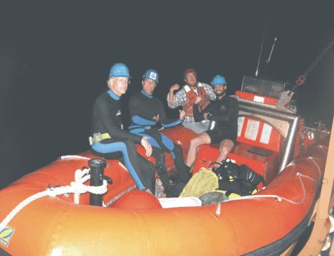
Figure 2. Larry Madin, Erich Horgan, Phil Pokorsky, and Keegan
Plaskon ready to begin a night-time blue-water dive [Photo by P.Wiebe].
20 April 2006: The first official deep tow of station #3 started around midnight on the 19th with the deployment of the 10-m MOCNESS under good sea conditions (winds in 10 to 12 kt range). The launch was a bit difficult at the start, but ultimately the frame rolled down into the water fairly smoothly and soon the net was headed down to depth. During the night there was a wind shift and light winds around 5 to 8 kts began from the north (0°). In the early morning it was cloudy with rain squalls in the area and cooler temperatures (20.73° C). It was raining lightly when the MOC-10 tow #3 came on board very nicely around 0930 on 20 April. This tow was also discovered to have problems. In pulling in the nets, it was found that the cod-end from net three had been lost in spite of the fact that the fasteners had been rubber-banded, which has been the standard way to prevent bucket loss. In addition, the tab on net bar #3 that had been fabricated by the engineers again broke, so that the net bar for net 3 dropped when net 2 was closed and it never fished. This opened net four prematurely. Later in the day, the broken tab fixture was repaired by the engineers, who made it more robust. The catch in the rest of the cod-ends, while sparse, proved to have another set of very interesting deeps sea invertebrates and vertebrates. One interesting species was a mysid in the Gnathophausia group. There are several well-known species, but this did not appear to be any of them. In addition, there appeared to be no contamination by animals living shallower in the water column or very little. The modifications made to the system appeared to have worked.
The 1-m MOCNESS was next up. It went into the water about 1130, but at 70 m depth, the deck unit lost connection with the underwater unit and nothing would bring it back. So the system was brought back on board. After a series of tests that determined that the cable was OK, the underwater unit was switched with the one on the MOC-10. The tow was started again about an hour later. This time the underwater unit worked fine and a complete set of samples was obtained in the upper 1000 m. The net came on deck about 1600. Such were the gremlins out there, that when the unit that failed was bench-tested, it worked.
Larry Madin, Erich Horgan, and the two crew divers left the ship about 1630 for the next in a series of blue-water dives, as the afternoon watch processed the MOC-1 samples. While the divers were away from the ship in the zodiac, some surface ring net tows were taken by hand. All went well with the dive and the divers returned with more wonderful animals around 1730.
The last events at station #3 were night 1-m and 10-m MOCNESS tows to 1000 m and 5000 m respectively, and a ring-net tow to 200 m. All of these tows were accomplished successfully. The 1–m system was towed early in the evening followed by the ring net tow. The 10-m system, which was deployed at midnight, came up at 1130 on the 21st. This time all the nets fished their intended depths (5000 to 4000, 4000 to 3000, 3000 to 2000, and 2000 to 1000 meters) and the samples showed little or no contamination. This was a perfect ending to a station that started off poorly.
The Ron Brown got underway for station #4 just after noon on the 21st of April in light winds, calm seas, warm air temperatures, and clear skies. Because diving conditions were extremely good and the animal collections were going very well with this technique, a blue-water dive was scheduled for 1330. The divers returned about 1500 and reported that while animals were sparse, they again collected some interesting radiolarians and siphonophores. The remainder of 21 April was spent steaming under very nice sea conditions. The work on board in the laboratories continued unabated.
22 April 2006: The steam to Station #4 (20° N; 55°W) took about 32 hours under mostly clear skies with only a few clouds. In the early morning of 22 April, winds 10 to 15 kts were from the northeast, the sea surface temperature (SST) was 25.56° C, and the air temperature was slightly cooler (24.1° C).
Throughout the day, the investigators worked in the main lab identifying zooplankton and in the sequencing lab they continued to prepare and sequence identified species. During the afternoon of the 23th, the second session in the seminar series was held with Larry Madin, Hege Hansen, and Tracey Sutton giving the talks. Larry talked about the Liquid Jungle Laboratory, which is a new tropical laboratory for marine and terrestrial research on the Pacific side of Panama. There is a shore-side wet lab in addition to lab space in the main building up on an island hillside, small boats for access to the coastal waters, and a newly installed cabled underwater observatory just offshore. Hege talked about the deep-sea shrimps that were collected on the Mar-Eco cruise to the mid-Atlantic ridge on the R/V GeoSars in summer 2004. She compared the species caught on that cruise with those collected on this one. So far she has found only one species additional to those collected on the ridge cruise and only a single northern species is currently lacking from our current collections. Tracey gave an overview of the groups of deep-sea fish that exist and talked about those that he was finding in our samples. He has found several rare species and one or two that are probably novel. The talks were split into two sessions because the ship’s personnel had a safety meeting at 1415 that went until about 1515.
After dinner, the 10-m MOCNESS was made ready for the next watch to launch and tow. The cod-end buckets were attached to the nets and the nets arranged so that they could be deployed off the stern easily. In addition, some repairs to the newly fashioned trawl deflector flaps were made.
23 April 2006: We arrived at Station #4 about 0035 on 23 April and started the work with a vertical Reeve net tow to 200 m. This was followed by a 10-m MOCNESS tow. The bottom of the tow was at 4500 m instead of 5000 m because of the very rough topography in the area. The SeaBeam bathymetry data showed that there were substantial ridges and valleys in the area and our tow line cut across them. The broken strand of 0.68" conducting cable at about 4700 m that was taped after the last tow, came loose after the tape had worn off going through the traction winch and had to be re-taped when it came past that spot going out and coming back in, but this did not interfere with the haul. The system came up and on board at 1245. As the nets were being hauled in, the catch in the buckets were initially examined. There was a spontaneous “OOOOH!!” as a large dragonfish was found in the bucket of net 4 (2000-1000 m). After examining it carefully in the laboratory Tracey Sutton concluded it was probably a new species, and might even represent a new genus. The catch also contained some lovely large red prawns. Not only was this an excitingly spectacular haul, but also once again the nets had fished properly.
A daylight blue-water dive took place in the early afternoon under light winds (~8 kts) from the northeast and sunny skies. The divers returned with only a few animals. The dominant organisms were phytoplankton, the nitrogen fixer Trichodesmium and mats of Rhizoselenia. The zooplankton were sparse.
While the divers were out, the 1-m MOCNESS was set up for a tow. The cable termination was changed from the MOC-10 to the MOC-1 and then the underwater unit moved to the MOC-1. About 1520, after a deck check to make sure the electronics and sensors were operational, the net entered the water and the tow began. This tow went fine, except that a collar came off of net 3 and the catch was lost along with the bucket.
Russ Hopcroft and Barbara Costas did a series of net tows and water collection casts, while the 1-m MOCNESS was prepared for a second evening tow. The net system went in smoothly from its position within the back of the MOC-10 frame. The tow, which came on board around 0130 on the 24th, concluded successfully with more interesting animals in the catch. These included a small tropical squid in the surface sample that Dhugal Lindsay knew existed, but had not seen before.
24 April 2006: In the wee hours of 24 April, the divers went out in the RHIB for a night dive in waters that were now around 26.5° C. Again the take was sparse, reflecting the oligotrophic nature of the station area, but they did collect two very interesting delicate ctenophores, Beroe mitrata, and Thalassocalyce inconstans. Larry Madin and Richard Harbison discovered and named the latter species some time ago. The genus means “cup of the sea” after its shape and inconstans because it is in constant motion. Both individuals were still alive in the evening of the 24th and were the subject of observation and photography, prior to being submitted for sequencing.
A 1/4-m MOCNESS tow was scheduled as the last item to be done at Station #4, but the underwater unit again proved to be unreliable on the deck and so the tow was scrubbed. The ship got underway for the last station (#5) about 0400.
Steaming during the day again gave the investigators an opportunity to catch up on the laboratory investigations of the samples collected at the previous station. There was also a concerted effort to update the CMarZ web site and to add additional photos of people and gear at work on the cruise. It was pleasant steaming weather with sunny skies sprinkled with puffy clouds, winds from the east (90°) at about 15 kts giving rise to some white caps and choppy seas on top of an underlying swell. Both the sea and air temperature was around 26° C.
At 1400 on the 24th, a subset of the scientific party (Martin Angel, Larry Madin, Rob Jennings, Russ Hopcroft, Tracey Sutton, and Peter Wiebe) met in the Chief Scientist’s cabin to take part in a press conference call organized by Fred Gorell of NOAA. In preparation for the call, two photos were put on the web of two of the first zooplankton (the copepod, Paraeucalanus attenuatus and the pteropod, Clio pyramidata) collected on the cruise that were in the first group sequenced at sea. In addition, a photo of Paola Batta Lona “operating” the sequencer was also posted on the web. Reporters on the call included Christina Reed, a freelance science writer, Peter Spotts of the Christian Science Monitor, Warren Wise of the Charleston (SC) Post & Courier, and Noel Anenberg, who writes a children's / educational series for LA Times. In addition, there were several others taking part in the conference call including Ann Bucklin, the CMarZ lead investigator and a co-PI on this OE project, responsible for the shipboard sequencing activities. The conference call lasted about 75 minutes and covered the overall rationale for CMarZ and the cruise objectives. Questions from the reporters then framed the remarks made by our group of scientists about what we had already learned and how the sequencing information would ultimately be used. The session was tape-recorded by NOAA.gov and would be used for production of a story to be podcast. Coincident with the press conference was the third and last Fire and Emergency Drill, from which the participants were excused.
A schedule of MOCNESS tows, blue-water dives, and other net tows and water collections was prepared in the late afternoon for the first day and a half at Station #5. The early evening was spent setting up the 1-m MOCNESS for a tow after the ship arrived on station the next morning.
Then late in the evening around 2300, the third in the seminar series took place. This late hour was chosen because this was when most of the scientists from both watches, i.e. the midnight to noon and noon to midnight, were awake. With the last station quickly approaching and the end of the cruise in sight, there was an increased impetus to make the most of the time remaining. Barbara Costas provided an introduction to the ciliates and in particular the groups that include tintinnids, oligotrichs, and other choreotrichs. She described her work on tintinnids (small ciliate microzooplankton) and the difficulties involved in using the classical methods to preserve and identify them . She has been developing molecular methods to determine species identities, and has found that a number of forms previously described as distinct species appear to have very similar genetics and may not be separate species. A library of ciliate genetics is being built and is at the point in some areas where bulk DNA analysis can be used to track the presence and perhaps the abundance of the different species. Rob Jennings described the steps carried out by Team DNA in the processing of the animals in the sequencing lab. This involved extracting the DNA, amplifying it, running the sequencing reactions, and then running the product on the sequencer. He described how to resolve the data from noise in the reaction by sequencing a forward strand and a reverse strand. Once the sequence has been finalized, the next step was to compare it to known sequences in the bank of sequences to see if the sequence matches one for a known species. Since the cruise began, about 500 species have been submitted to the lab for sequencing and there have been 775 specimen extractions. [Note: These numbers have gone up since station #5 was not included in the estimates]. Russ Hopcroft gave a tutorial on larvacean diversity and ecology. Like the tintinnids, the larvaceans are extremely fragile animals and are difficult to collect intact. They make an elaborate external feeding structure that they use and then discard when it gets clogged up. This may happen as often as 14 times per day. Russ described the house structure, which is unique to each species and therefore can be used to identify the species. There are 3 families, 15 genera, and 69 known species. On this cruise, he has collected fewer larvaceans than expected.
25 April 2006: The Ron Brown arrived at Station #5 around 0830 on 25 April with the decks wet from some early morning rain showers. Unlike the previous few days, the skies were cloud covered. Still the winds were light (5 to 8 kts from the east southeast) and the air warm (25.9° C) and humid. The sea surface temperature was the warmest experienced on this cruise (27.147° C).
Almost immediately there was a net in the water. Russ Hopcroft deployed his Reeve net for a tow to collect larvaceans. In this tow were several larger species of larvaceans that he was expecting to encounter, but had not done so until now. The 1-m MOCNESS went in about 0915.
In the area of station 5, there are physical structures in the water column between 200 and 500 m known as “thermohaline staircases”. When a plot of temperature or salinity versus depth is made, distinct steps in the profile are visible wherein there are zones of ten meters or more of isothermal and isohaline water and then narrow transition zones where both temperature and salinity change abruptly until there is another step. The zones of constant temperature and salinity are active mixing zones as demonstrated by work that Ray Schmitt and colleagues had done in this area some years ago. The staircase structure might also be an area of unique biology, but this has not been previously studied. Knowing that there was the possibility that the staircase structure might be present, we looked carefully at the data from the first tow as it was in progress. The tow went smoothly and during the downcast a plot of the temperature and salinity structure showed that indeed there was a staircase structure in the same depth zone that Schmitt had observed in 1985.
At the end of the tow, while the net was approaching 25 m depth, the winch overheated and shut down. It took a relatively short time for the engineers to investigate the problem and to start the winch operating again. The last net then sampled the upper 25 meters and the net came on board about 1238.
The divers went in around 1300 with winds in the 12 to 15 kts range. They came back with a real beauty of a collection of jellyfish, siphonophores, and salps. This station was very different from the previous two because of the rich surface life they encountered.
In the late afternoon, ring net towing primarily for larvaceans and foraminifera, and water collection for microzooplankton (tintinnids) were carried out. At dusk, the second 1-m MOCNESS was started. This tow was very successful. All the nets opened and closed where intended and the catches were quite good. There were no problems with the winch this time. Once the 1-m net was secured, the cable termination and underwater unit from the 1-m system were moved to the MOC-10, the buckets installed, and the nets arranged for deployment. This took about an hour. By 2200 the MOC-10 was heading down to depth.
26 April 2006: Some twelve hours later at 1000 on 26 April, the trawl re-appeared at the surface. It had caught a wonderful assortment of animals, especially fish. Tracey Sutton was particularly pleased. Martin Angel was busy trying to increase his inventory of ostracod species and exceed his previous inventory compiled for the Eastern Atlantic. Already at the start of this station he had identified nearly a third of the known species of planktonic ostracods. Net one, the first to be fished as the system returned from 5000 m to the surface, was ripped up a bit on the starboard side and a support rope was ripped off the seam to which it had been attached. It is a mystery how this happened.
Shortly after, the 1/4- m MOCNESS was returned to service by using an old 16-bit electronics unit that was brought on the cruise in case other units failed to operate properly. This tow to 500 m went OK, except that the flowmeter stopped working during the net system’s return to the surface. Water filtered for some nets will thus have to be calculated by time the net was open and distance traveled These samples caught with very fine mesh nets (64 um) were primarily used by those investigators interested in microzooplankton.
The second 10-m MOCNESS tow of station #5 started in the early afternoon under fair skies with winds a steady 12 to 15 kts from the east northeast (82°) and tropical air (26.22° C) and water (27.19° C) temperatures. Around 1900, the MOC-10 reached within 200 m of the bottom (~5200 m) with more than 7000 meters of wire out. The rest of the evening was spent flying the MOC-10 up from 5000 m. The tow took longer than expected. The net came up too fast on its own accord to haul wire in quickly, so a good portion of the tow was spent coming in at 10 or 15 m/min.. The first net fished from 5000 to 4000 m. On this last MOC-10 tow, it was decided to use the last net to fish the upper 1000 m and use the other three to cover the 5000 to 1000 m range. The group was really interested to see what large-ish animals might be captured in the near-surface zone with the big fine-meshed nets.
27 April 2006: At midnight on the 26th, when the science watch changed, Larry Madin came in to take over the “flying” of the MOC-10. There was some discussion about whether the nets had opened and closed where intended because no significant angle change had been observed when the net system was sent the command to close one net and open the next. When the net system finally came on board about 0330 on the 27th, the concern disappeared. All evidence suggested that the nets opened and closed where intended and the catches were pretty spectacular. Contamination was minimal. Francesc Pagès was excited because previously he had been catching a particular transparent jellyfish about 5 cm in diameter in the 1-m MOCNESS collections that had very few distinguishing characteristics and was an undescribed species as far as he could tell. In the 1000 to 0 net, a much larger individual was caught and it had characteristics that he could now use to make a description. Also Dhugal Lindsay was happy with the squid collection. Several species that had not been caught earlier were in the sample including a Vampyroteuthys. Martin Angel also found specimens of a species that he had been looking for. In addition, Russ Hopcroft gave Martin another ostracod not yet seen on the cruise from a Reeve net collection made soon after the trawl was on board (from 0415 to 0445). So the last station was ending with a flourish.
The 1/4-m MOCNESS tow began around 0600, under cloudy conditions and winds 13 to 18 kts from the east. A few rain squalls moved through the area. This tow was used to sample a special series of depths for Colomban de Vargas and Yurika Ujiie to look at how the vertical salinity and temperature structure in the upper 300 m might be affecting the foraminifera. This targeted depth sampling was based on the information from the down trace and from earlier tows. The 1/4-m tow came back on board about 0900 with samples that were a bit disappointing to Colomban because the catches were fairly sparse and there were few foraminifera.
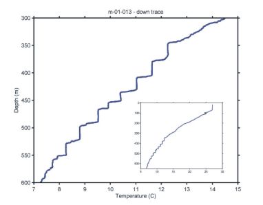 Figure 3. The
temperature profile from the last 1-m
MOCNESS tow of the CMarZ cruise showing the staircase structure.
Figure 3. The
temperature profile from the last 1-m
MOCNESS tow of the CMarZ cruise showing the staircase structure.The last tow of the cruise was made with the 1-m system. It was targeted at the staircase structure mentioned above, which showed prominently on every tow at this station that went below 300 m (Figure 3). Nets were opened and closed so that one fished in an isothermal/isohaline (mixed) zone and then the next in the interface between it and the mixed zone just above. We successfully fished 4 mixed zones and 4 transition regions starting about 550 m below the surface and ending about 400 m.
Over the last three days, Team DNA received more identified specimens for sequencing and also a few more unidentified forms that might be undescribed. The total number of identified specimens in the bank topped 1000. More than 400 sequences had been run and it was anticipated that there would be more than 100 good species sequences by the end of the cruise. Many of the other sequences may turn out to be usable or may need more work to make them good. The nature of the sequence would determine what additional steps might need to be taken, like running an additional PCR under different conditions to optimize the sequence reaction. There is more work to sequencing than simply extracting the DNA, amplifying it, and then running it through the sequencer to get the sequence. Having to repeat steps with different conditions is typical.
With the last over-the-side sampling completed around 1500 on the 27th of April, the R/V Ron Brown set sail for San Juan, Puerto Rico.
28/29 April 2006: During the two day trip to San Juan, the activity of the science party focused on packing up all the gear and getting it ready for off-loading and shipping on the day the ship reached port. In addition, the investigators wrote up sections of the cruise report.
At 1030 on the 28th, there was a conference call with CoML media relations lead, Terry Collins. Included in the call were Martin Angel, Larry Madin, Rob Jennings, Tracey Sutton, Russ Hopcroft, and Peter Wiebe. Also Ann Bucklin and Fred Gorell were present from a distance. Discussion centered on what was going to be the focus of the CoML press release about the cruise and its findings.
During the morning of the 29th (around 0900), there was a final 45 minute blue-water dive involving all of the authorized divers on board to inspect the hull of the Ron Brown. Later in the evening after we arrived back in the US EEZ a net tow was taken to obtain live zooplankton for video imaging by Russ Hopcroft to be used as part of the press material package on the CoML web site.
The 20' shipping container van on the ship was loaded by mid-afternoon on the 29th of April and the remaining gear was assembled in totes and boxes for off-loading and packing in a second van that was to be on the Coast Guard dock in San Juan.
30 April 2006: The R/V Ron Brown entered San Juan, Puerto Rico harbor about 0800 on 30 April. With the tying of the lines on the Coast Guard dock in the Old Town area of San Juan, this CMarZ cruise came to an end. Off-loading of the science gear began shortly after the ship was tied up. By noon, the second van was loaded and ready for shipment back to Woods Hole, Ma.
This CMarZ cruise was a remarkable expedition that brought together classical taxonomists and gene sequencing experts to collaborate at sea and produce impressive results in just three weeks. Zooplankton and fish samples were obtained from 5000 m to the surface at five stations distributed from 33.5 N to 14 N in the western North Atlantic Ocean. From these samples, the investigators identified between 500 and a 1000 species, and they provided more than a 1000 specimens to the DNA lab on board the ship for sequencing. For several taxonomic groups, a significant fraction of the known species were collected and identified. For example, 65 species of ostracod were identified by Martin Angel, representing nearly half of all 140 known ostracod species in the North Atlantic Ocean. Six of the ostracod species are not yet described in scientific literature. Nearly all of them were submitted for sequencing and the first DNA barcode for a planktonic ostracod was obtained on this cruise. More than 40 species of molluscs (pteropods, heteropods, etc.) were identified and more than 100 species of jellyfish, several of which may be undescribed. Several hundred species of copepods were identified and more than 100 species of fish, many rarely caught, and two of which may be undescribed. In addition, several groups brought photographic equipment on the cruise that enabled hundreds of high resolution digital photographs to be made of many of the zooplankton species identified and submitted for sequencing. Russ Hopcroft in particular made many photos that were put up on the web site during the cruise.
Having a gene sequencer and associated DNA laboratory equipment and personnel on board made it possible for a level of interaction between taxonomic specialists and molecular biologists that is seldom achieved in any other setting. The high productivity in terms of the identification and sequencing of known and unidentified specimens was the result of the very positive interactions that occurred while at sea. In spite of the difficulties encountered in MOCNESS sampling, the goals of the cruise were met and overall results were successful.
MOCNESS and OTHER SAMPLING, and SAMPLE PROTOCOLS
Zooplankton and micronekton were quantitatively sampled throughout the water column using a 1/4-m, a 1-m, and a 10-m MOCNESS (Multiple Opening/Closing Net and Environmental Sensing System; Wiebe et al., 1985; Figure 4). The MOCNESS telemetered data continuously to the ship, including depth, temperature, salinity, horizontal speed, and volume filtered. This allowed on-the-fly adjustment of sampling depths or times, and completion of a continuous series of stratified hauls in a relatively short time. All data were recorded electronically for subsequent analysis.
 Figure 4. The
three MOCNESS’s used on the CMarZ
RB06-03 cruise to the Northwestern Atlantic Ocean. Note
the net bar and deflector flaps on the MOC-10 developed on
the cruise to prevent contamination of the samples.
Figure 4. The
three MOCNESS’s used on the CMarZ
RB06-03 cruise to the Northwestern Atlantic Ocean. Note
the net bar and deflector flaps on the MOC-10 developed on
the cruise to prevent contamination of the samples. The MOC-10 carried 5 separate nets; the mesh size of the nets was a combination of 3 mm and 335 µm mesh. Net 0 had 3 mm mesh and nets 1 to 4 had 335 µm mesh nets of special design that were fabricated for this cruise. In addition, during the cruise, deflector side flaps and net bar flaps were constructed to prevent contamination of the deep samples from plankton in other strata, especially those closer to the surface (Figure 4). The MOC-10 was launched, towed, and recovered through a stern A-frame with the ship maintaining a speed of 1.5 to 2.5 kts. The trawl was deployed with the first net open (3mm mesh) down to the deepest depth desired, normally 5000 m. It was closed at that point, and subsequent nets (335 um) were opened at desired depths as the trawl was hauled obliquely toward the surface. Thus, one MOC-10 net sampled from the surface to the bottom and the other nets normally sampled ~1000 m intervals from the bottom up to a depth of 1000 m (Figure 5).
Above 1000 m, vertically-stratified sampling was done using a 1-m MOCNESS equipped with 9 nets with 335 µm mesh. In addition, a ¼-m MOCNESS with 0.64 µm mesh was used to collect foraminifera and other micro-zooplankton in the upper 500 m (Figure 5). The use of the large trawl below 1000 m enabled large volumes of water to be sampled (tens of thousands of cubic meters) to compensate for the very low abundance of species that occur at bathy- and abyssopelagic depths. The smaller 1-m and 1/4- m MOCNESS’s provided adequate sample sizes in the upper 1000 m.
Several other nets were used for surface or near surface zooplankton collections. A Reeve Net consisting of a ½-m ring net attached to a large-volume cod-end was used to collect fragile gelatinous animals and microzooplankton in the upper few hundred meters. These tows were made opportunistically. Other very fine mesh (5µ and 10µ) ring nets deployed by hand were used to collect microzooplankton during periods when the blue-water dives were taking place.
 Figure 5. The general towing and sampling strategies
used for the MOCNESS’s.
Figure 5. The general towing and sampling strategies
used for the MOCNESS’s.
2.0 Blue-water SCUBA diving for gelatinous zooplankton.
Collection of living or intact specimens of gelatinous zooplankton is difficult with nets or trawls because the organisms are usually damaged and sometimes destroyed. During the last 30 years, the technique of blue-water diving to make observations and collections of these fragile animals by SCUBA has been developed and this technique was used on this cruise. A group of (usually) 4 divers worked from a small inflatable boat launched from the ship. They were connected by 10 m long tether lines to a central line hanging down from the inflatable and manned by a safety-diver who watched over the others. Each diver moved about within a 10 m radius to locate, observe, and collect free-swimming gelatinous animals. The technique was only semi-quantitative, but allowed collection of live and undamaged specimens, as well as in-situ photos of behavior. Organisms were collected in simple wide-mouth jars and returned to the ship for further study. The same technique was used at night, with the addition of underwater flashlights or headlamps. During this cruise a day and a night dive was planned for each station.
A thirty-liter Niskin bottle was used to collect water for tintinnid analysis and for use with other work with microplankton. The depths selected for sampling were generally based on the water column temperature and salinity structure.
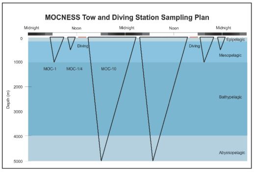
An idealized scheme for sampling at each station was approximated that enabled replicate tows with each MOCNESS to be made during an approximately 48 hr period (Figure 6). MOC-10 tows generally took 10 to 12 hours to complete, MOC-1 tows took about 3.5 hours, and MOC-1/4 tows took about 2 hours. In addition, a 2-hour time block was allocated for two blue-water dives. Not shown on this scheme was time for opportunistic sampling with ring nets or water collection with the Niskin bottle. In reality, neither replicate samples with all net systems nor blue-water dives were obtained at all the stations, because of time and weather limitations, and gear malfunctions.
5.0 Sample Processing Protocol.
Samples collected with the MOCNESS’s were processed using a standard protocol (Figure 7).
On Deck: With completion of the tow, the nets were immediately washed with seawater as they were pulled on deck and the plankton still in the nets carefully moved into the cod-end. The cod-ends were placed in buckets with ice packs to cool the samples and moved expeditiously into the walk-in cold room to await analysis.
Ship-board laboratory processing:
Specimen removal: One by one the cod-ends were taken into the wet lab for digital photographing, and the picking and removal of large individuals of 1) gelatinous forms, 2) fish, and 3) macrozooplankton/nekton. Pickers described what was being removed and a recorder logged the information. The specimens removed were placed in numbered jars, shell vials, or dishes and the recorder wrote down all specimen information on the data sheets provided, linking the container number to specimen and collection data. This was done so that the actual taxonomic composition and species count for each sample can be reconstructed. The removed specimens were subject to a variety of procedures including further identification, dissection, preservation (in alcohol, frozen nitrogen, or formalin as appropriate), or taken for photographic imaging prior to preservation.
Sample splitting and preservation: Within a few minutes of arrival, the stratified samples (with most large gelatinous forms, fish, and macrozooplankton/nekton removed) were passed to the individuals responsible for splitting the samples (Figure 7). Generally ½ (split A) was preserved in formalin for future studies, including biomass estimates (e.g., displacement volume), species counts, and other quantitative analyses. The other half was split again with ¼ (split B) for live picking in the main lab and subsequent preservaton in alcohol for later taxonomic analysis. The other ¼ (split C) was immediately preserved in alcohol. After picking, the integrated sample (net 0) was generally split into two halves with one preserved in alcohol and the other in formalin. Picking of foraminifera from the live split took a long time, so this fraction was kept in the the cold room and often not preserved in alcohol for several hours. Condition of these samples is questionable.

Figure 7. Schematic drawing of the protocol for
processing
zooplankton
samples on the CMarZ cruise.
Sample analyses: Species were identifiedby the taxonomic experts on board. Several individuals of each identified species were placed in a labeled vial and submitted to the DNA lab for at-sea DNA extraction, PCR amplification of target genes, and sequencing (with a few specimens retained as vouchers). Samples and specimen numbers were entered into the CMarZ Specimen Log, an ACCESS database. Representative specimens of many species were digitally photographed before preservation and some were photographed after preservation.
Specimens of the skeletonized protists were recovered from epi- and mesopelagic samples using simple decantation processes. The taxa of interest were manually sorted under a dissecting microscope immediately after collection. The isolated cells were cleaned in filtered sea-water using micro-brushes, and put into individual tubes containing 100 μl of GITC buffer. This buffer has been developed in the de Vargas laboratory and allows extracting the nucleic acids from the organisms while preserving their micro-shell. The material was stored at -20°C before further analyses. Total DNA was extracted according to protocols developed by de Vargas et al.
WATER COLUMN STRUCTURE AT THE STATIONS
The Station locations (Figure 1), which ranged from the Northern Sargasso Sea to the tropical waters east of the Windward Islands, provided contrasting physical settings for the zooplankton collections. In the Northern Sargasso Sea, the “eighteen degree water” was present from near the surface (~40 m) to more than 400 m deep with only a shallow mixed layer of slightly warmer water at the surface (Figure 8). The main thermocline and halocline occurred between 500 and 1000 m below which temperatures gradually decreased from around 5° C to below 3° C at 5000 m. At station 2, a similar structure was present, although the surface layer was warmer (~20° C) and there was a distinct gradient in temperature and salinity in the “eighteen degree water” zone. The upper water column T/S properties at station 3 were distinctly different with lower salinity water at the surface increasing to a maximum around 100 m, and a much warmer surface temperature (~24° C). In addition, the zone of nearly isothermal and isohaline water seen at the northern stations was no longer present. Instead, below 100 m there was a steady decrease in temperature and salinity to about 900 to 1000 m and then a more gradual decrease in temperature. Salinity reached a minimum at about 900 m and then increased down to about 1200 m before gradually decreasing to 5000 m.
The pattern of low salinity at the surface, a peak at ~100 to 140 m, a minimum at 800 to 1000 m, a secondary maximum around 1400 m, and then a gradual decrease to the sea floor was observed at stations 4 and 5 in increasingly exaggerated form (Figure 8). Sea surface temperature also increased to the south with Station 5 having surface temperatures around 27° C. In addition at station 5, the staircase formations between 250 and 550 m were present as described in the narrative (Figure 3). An explanation for the origin of the water seen in the area sampled at stations 3 to 5 was provided by Ray Schmitt (WHOI) while we were at sea.
“The low salinity water at the surface originates in near equatorial latitudes, where rainfall exceeds evaporation under the Intertropical Convergence Zone (ITCZ). Basically it’s the water that evaporated under the trades coming back down. The Amazon outflow is also important in this freshwater supply. ... The salinity maximum at ~150 m depth is coming from the Northeast. It is formed from the surface waters that have experienced high evaporation under the trades and been transported to the north in the surface Ekman layer. There is a region at ~25 N in the eastern Atlantic where the salinity maximum is at the surface, this water is subducted and carried southwest in the gyre circulation to [this area]. Georg Wust called it the Subtropical Under-Water (SUW). Farther down at about 800 m depth, [there is] the salinity minimum associated with the Antarctic Intermediate Water (AAIW). It’s coming from the south, as part of the thermohaline circulation. Freshness originates from precipitation in the Southern Ocean.
So it’s a layer cake with surface freshness from the South, SUW from the North and AAIW from the South. The salinity gradient in the main thermocline between the SUW at ~37.2 and the AAIW at ~34.8 may be the strongest large scale unstable salt gradient in the world. And thus its propensity for forming these salt finger staircases.”
1.0 Blue-water Diving (Larry Madin)
Blue-water, or tethered open-water, diving is a simple technique that allows observation, photography, and collection of undamaged live zooplankton, particularly larger gelatinous forms that are commonly damaged or destroyed in nets. During the CMARZ cruise, 8 dives were made by Larry Madin and Erich Horgan, assisted by RV Brown crew members, Lt. Liz Jones, Ens. James Brinkley and 1st Asst. Engineer Keegan Plaskon. Dives were supported by the RV Brown’s RHIB workboat, driven by Phil Pokorsky. We made at least one dive at each station, with 5 during daylight and 3 at night (Table 1).
On this cruise the main dive objective was to collect gelatinous animals for identification and DNA bar-code sequencing, as these forms are less likely to be represented in net collections. During the dives we collected approximately 260 individuals of 42 species (Appendix 2). This included 4 species of medusae, 13 of siphonophores, 6 of ctenophores, 7 of molluscs, 10 of thaliaceans, and a few others. In the oligotrophic waters of Stations 4 and 5, we encountered numerous colonial radiolarians and Trichodesmium. In general the abundance of large macrozooplankton on these dives was fairly low, consistent with the low abundances of other zooplankton sampled with the nets.
Some notable findings included two specimens of the epi- and mesopelagic ctenophore Thalassocalyce inconstans, a specimen of the siphonophore Halistemma cupulifera that had caught a leptocephalus (eel) larva, and a surprisingly high diversity of both siphonophores and Thaliaceans. Collected specimens were examined for taxonomic identification, morphological study and behavior, and then added to the group to be sequenced.
Collections of Thaliacea (salps, doliolids, pyrosomes) were rather sparse on this track, although 17 species were obtained either in the net tows, or more often, from the dives.
Net collected samples included:
1. Cyclosalpa polae (aggregate)
2. Thalia democratica (solo & aggregate)
3. Salpa cylindrica (solo)
4. Iasis zonaria (solo & aggregate)
5. Salpa aspera (aggregate)
6. Salpa fusiformis (solo & aggregate)
7. Helicosalpa virgula (solo)
8. Dolioletta gegenbauri
9. Doliopsis sp.
10. Doliolina sp.
11. Doliolum denticulatum
12. Pyrosoma atlanticum
13. Pyrosomella sp.
Most of these were in the shallower nets, and were only found in small numbers (1 to 4 of each).
Species collected during dives included:
Brooksia rostrata (aggregate)
Iasis zonaria (aggregate)
Salpa aspera (solo & aggregate)
Salpa fusiformis (solo & aggregate)
Salpa maxima (solo & aggregate)
Salpa cylindrical (solo)
Pegea bicaudata (aggregate)
Pegea confoederata (aggregate)
Dolioletta gegenbauri
Doliolina sp.
Pyrosoma atlanticum
All salps were identified and measured, and good specimens (mainly from dives) examined and photographed for anatomical details. These descriptions will become part of the detailed morphological information which will accompany the genetic data. A parallel project to develop a morphological and molecular phylogeny of the Thaliacea will be carried out by Madin and Bucklin over the next two years.
Table 1. Distribution of species by Station
Station 1 |
Station 2 |
Station 3 |
Station 4 |
Station 5 |
B. rostrata |
C. polae |
C. polae |
B. rostrata |
C. polae |
C. polae |
I. zonaria |
P. bicaudata |
D. denticulatum |
H. virgula |
I. zonaria |
S. aspera |
P. confoederata |
|
I. zonaria |
S. aspera |
S. fusiformis |
S. aspera |
|
P. confoederata |
S. cylindrica |
D. gegenbauri |
S. fusiformis |
|
S. fusiformis |
S. fusiformis |
D. denticulatum |
S. maxima |
|
S. maxima |
T. democratica |
Doliopsis sp. |
D. gegenbauri |
|
T. democratica |
D. gegenbauri |
|
Doliolina sp. |
|
D. denticulatum |
|
|
D. denticulatum |
|
|
|
|
P. atlanticum |
|
|
|
|
Pyrosomella sp. |
|
|
All species found at the 5 stations can be considered warm-water cosmopolitan forms. Although Station 3 appears to have the greatest diversity and Station 4 the least, the sample sizes are probably much too small to draw any real conclusions.
3.0 Planktonic Cnidarians (Francesc Pagès, Dhugal Lindsay, and Larry Madin)
Our main goal was to increase knowledge of the species composition and vertical distribution of planktonic cnidarians, mostly below 1000 metres depth. About 110 species have been collected, namely siphonophores (70 species), hydroidomedusae (30 species) and scyphomedusae (10 species). About 5 medusae have not been properly identified (nicknamed as Red Ball, Pegantha 24, Pegantha M, White Nausithoe, and Transparent Nausithoe) and some could be new species. One of the nicest and more interesting specimens is an epipelagic narcomedusan of the genus Pegantha (P. 24), whose 2 otoporpae (lines of cnidocysts) per marginal lappet bifurcate ending in 4 statocysts (sensorial organs), a splitting never before reported in any other narcomedusan.
The blue-water dives led by Larry Madin and Erich Horgan collected valuable specimens of rare and little-known species like the recently described siphonophore Lilyopsis fluoracantha (Haddock, Dunn and Pugh, 2005), but most of the specimens belong to species described a long time ago, such as Athorybia rosacea (Forskal, 1775), Rosacea cymbiformis (Chiaje, 1822), and Lilyopsis rosea (Chun, 1885).
The Ring net and the Reeve net proved to be excellent devices for collecting small-sized planktonic cnidarians. In particular, the examination of some early stages of hydromedusae that were collected will shed further light on the growth, development, and morphology of some multispecific genera like Podocoryna and Bougainvillia.
The MOCNESS-1, towed in the top 1000m, collected the greater portion of the specimens examined. Many species widely distributed in epipelagic warm waters were obtained, as well as some specimens of little-known mesopelagic siphonophores like Frillagalma vityazi Daniel and Halistemma sp.
Below 1000 m depth, the MOCNESS-10 collected several little-known species such as the siphonophores Nectadamas richardi (Pugh, 1992) and Lensia quadriculata (Pagès, Flood and Youngbluth, 2006). Likewise some specimens of the genera Apolemia, Erenna, and Bargmannia were also captured, but their specific identification require additional microscopic analyses.
It is too soon to estimate the amount of information obtained in comparison with the sampling effort spent. However, in our opinion, the number of species found is lower than was expected, especially below 1000 m depth where the number of specimens caught was very low, suggesting a rather sparse macro- and megaplanktonic community of gelatinous organisms. This is only partly due to the use of nets for the sampling, since results from other oceans (e.g. Southern Ocean) using similar devices have collected higher gelatinous biomasses. It is interesting to note that very few specimens of the scyphomedusan genera Atolla and Periphylla were collected. Both are common dwellers in the meso- and bathypelagic waters of the oceans.
Preliminary results from the so-called “Staircase Tow” (MOCNESS-1 Tow 13) carried out on 27 April at station 5 suggest some kind of species stratification along the hydrographic staircase. Twenty species of gelatinous zooplankton were collected, namely 13 siphonophores, 3 hydroidomedusae, 3 ctenophores and 1 salp. Only the siphonophore Abylopsis tetragona -a fast swimming species- occurred in the eight ranges sampled between 547 and 461 m depth. Two siphonophores (Lensia ajax and L. exeter) occurred frequently, but irregularly between net 1 (547-527 m depth) and net 8 (464-461 m depth). An increase in the number of species was observed in even-numbered nets (2, 4 and 8) where several species occurred only at single depth ranges. Net 8 collected the three dominant species plus 3 new ones, indicating the beginning of a shift towards more epipelagic species composition.
4.0 Ctenophores, Amphipods, and Cephalopods (Dhugal Lindsay)
Ctenophore forms that were identified from net samples included several cydippids belonging to the Haeckeliidae (Aulacoctena acuminata), the Bathyctenidae (Bathyctena chuni), the Pleurobrachiidae (Hormiphora palmata, Pleurobrachia sp.1), the Mertensiidae (Charistephane fugiens), and others. Lobates such as Kiyohimea usagi and Ocyropsis maculata maculata, the Cestoid Cestum veneris, and several Beroe species were also caught in net tows. Blue water diving allowed the collection of several individuals of the lobate Eurhamphaena vexilligera and the Thalassocalycid Thalassocalyce inconstans, in addition to some of the forms listed above.
Twelve species of amphipods were sorted from the live samples, most of them large Physocephalata that were easy to spot. Many more species will undoubtedly be found upon examination of the formalin and ethanol-preserved samples. More than half of the gelatinous organisms captured during the blue-water SCUBA dives were host to hyperiid amphipods at varying stages of development. In many cases it was impossible to identify the hyperiid embryos to species or indeed genus level due to their early developmental stages. Individuals were extracted from the canals or gelatinous matrix of their hosts and placed in ethanol for sequencing. This should allow determination of any species specificity in host/parasite relationships as a factor contributing to species diversity maintenance mechanisms in the pelagic zone. The paucity of species belonging to the Physosomata at meso- and bathypelagic depths may have been a consequence of the dominance of these ecosystems by small siphonophores rather than the larger cnidarians that usually host these animals. Submersible dives should be conducted in this area to directly assess the types and numbers of large ctenophore and cnidarian forms to compare with the data gained on amphipods by net systems such as the MOCNESS.
Thirteen species of cephalopods were identified in the MOCNESS samples. Of these, three were octopods (Cirrothauma murrayi, Bolitaena pygmaea, Tremoctopus violaceus), one was a vampyromorph (Vampyroteuthis infernalis), and the remaining nine were various squids belonging to at least five major groups (Bathyteuthids, Chiroteuthids, Cranchids, Histioteuthids, and Enoploteuthids). Many larval individuals were also sampled and these were recorded photographically, dissected to obtain tissue for DNA analysis, and preserved in formalin for subsequent taxonomic analysis. Sampling with larger trawls will be necessary to assess the true diversity of the cephalopod fauna at these sites, but the 335 micron mesh yielded specimens in immaculate condition, greatly simplifying taxonomic analyses.
5.0 Decapod Shrimp (Hege Øverbø Hansen)
Samples were analyzed from the 10-m and 1-m MOCNESS (MOC-10 and MOC-1). A total of 18 tows were analyzed for the presence of Decapod shrimp: 11 samples from the MOC-1 and 7 samples from the MOC-10 (Table 2).
Table 2. Tows with MOC-1 and MOC-10 that sampled Decapod shrimp at the five stations. |
||
|
MOC-1 |
MOC-10 |
|
Tow # |
Tow # |
Station 1 |
1, 2 |
1 |
Station 2 |
3, 4 |
2 |
Station 3 |
5, 7, 8 |
3 |
Station 4 |
9,10 |
4, 5 |
Station 5 |
11, 12 |
6, 7 |
A total of 366 individuals were sampled and analyzed from MOC-1 and MOC-10.
Dendrobranchiata
Within Dendrobranchiata three genera were identified but identification to species level was not done on these individuals (N=147).
Within Sergestidae, the genera Sergestes sp. and Sergia sp. were found. Within Benthesicymidae there were at least two different species of Gennadas but again, certain identification to species level was not made.
Caridae
All individuals within Caridea were identified to species level (n=219). A total of 19 species were identified, belonging to the families Oplophoridae (17 species), Pandalidae (1) and Pasipheidae (1) (Table 3). Most of the observed individuals belonged to the family Oplophoridae.
Table 3. Species found on the CMarZ Cruise 10 - 30 April 2006. Species that were sent for DNA sequencing are marked (x). |
||||||
Dendrobranchiata |
Caridea |
|||||
Sergestidae |
Benthesicymidae |
Oplophoridae |
DNA |
Pandalidae |
Pasipheidae |
DNA |
Sergestes sp |
Gennadas sp |
Acanthephyra purpurea (A. Milne Edwards) |
x |
Parapandalus richardi (Coutiére) |
Parapasiphae sulcatifrons (Smith) |
x |
Sergia sp |
|
Acanthephyra stylorostratis (Bate) |
x |
|
|
|
|
|
Acanthephyra brevirostris (Smith) |
x |
|
|
|
|
|
Acanthephyra curtirostris (Wood Mason) |
x |
|
|
|
|
|
Acanthephyra microphthalma (Smith) |
x |
|
|
|
|
|
Systellaspis braueri (Balss) |
|
|
|
|
|
|
Systellaspis debilis (A.Milne Edwards) |
x |
|
|
|
|
|
Systellaspis pellucida (Filhol) |
|
|
|
|
|
|
Systellaspis cristata (Faxon) |
x |
|
|
|
|
|
Hymenodora gracilis Smith |
|
|
|
|
|
|
Hymenodora glacialis (Buchholz) |
x |
|
|
|
|
|
Meningodora mollis Smith |
x |
|
|
|
|
|
Meningodora miccyla (Chace) |
x |
|
|
|
|
|
Meningodora compsa (Chace) |
x |
|
|
|
|
|
Ephyrina figueirai |
|
|
|
|
|
|
Notostomus gibbosus (A.Milne Edwards) |
|
|
|
|
|
|
Oplophorus spinosus (Brullé) |
x |
|
|
|
Species richness of Caridae tended to increase with lower latitudes (Table 4).
Table 4. Number of different species found at the five stations with Latitude. |
|||||
|
Stations |
||||
|
1 |
2 |
3 |
4 |
5 |
Latitude |
33.5 |
30 |
25 |
20 |
14 |
Number of species |
5 |
10 |
6 |
10 |
13 |
Most of the individuals sampled were juveniles with a carapace length of less than 13 mm. However, some adult individuals were caught and some of these carried eggs on their pleopods (Parapasiphae sulcatifrons, Systellaspis debilis, Oplophorus spinosus, Acanthephyra purpurea and A. stylorostratis). For the first three of these species there seems to be a strategy towards eggs that are larger in size and fewer in number. The two latter species had smaller and more numerous eggs. A. purpurea and A. stylorostratis carried eggs that were developed to a stage where visible larvae could be seen within the eggs and were probably close to hatching.
Thirteen individuals were sent for DNA sequencing (Table 3).
Our main objective for participation on this cruise was to extend our knowledge of the distribution and biodiversity of pelagic shrimp in the deep zones of the Atlantic Ocean. Our goal was to identify all the sampled individuals within the Caridea while on board, and this goal was achieved. Specimens belonging to the suborder Dendrobranchiata were not identified to species onboard. However, post-cruise species identification by experts is possible through the MARBEF Taxonomy Clearing System/MAR-ECO.
Both the taxonomic and molecular results of the decapod shrimp from this cruise will be compared with previous results from the 2004 MAR-ECO cruise on the northern mid-Atlantic ridge. This will provide new knowledge on vertical and latitudinal variations in distributions, species composition and population structure of pelagic shrimp.
6.0 Mysids (Saramma Panampunnayil)
Five stations were sampled between 33° and 14° N and 70° and 54° W. At each station samples were collected using 1/4-m MOCNESS (upper 500m), 1-m MOCNESS (9 nets, upper 1000m) and 10-m MOCNESS (5 nets, down to 5000m), both day and night. Each sample was split. 50% was preserved in 5% formalin for silhouette analysis and later taxonomic analysis; 50% was preserved in alcohol for taxonomic analysis on board and removal of identified species for barcoding.
Mysids were picked out of the samples preserved in alcohol and identified.
MOCNESS 10: Bathypelagic Mysids. 8 species were recorded.
● Eucopia grimaldii was the most common species and occurred throughout the sampling area and was represented by all life stages (adult and young males, females and juveniles).
● Eucopia unguiculata, though a widely distributed and abundant bathypelagic mysid, was encountered at Station 5 only.
● Eucopia sculpticauda was present throughout with high representation at Station 5.
● Gnathophausia gigas. Two individuals, probably immature, measuring 57 and 100mm were recorded from Station 1 and Station 5.
● Gnathophausia sp. Two specimens from Station 4 (to be identified later).
● Lophogaster sp. Two specimens from Station 3 and Station 4 (to be identified later).
● Chalaraspidum alatum, a single adult male from Station 5.
● Boreomysis microps. This widely distributed bathypelagic form was represented by a single adult male at Station 1.
MOCNESS 1: 3 species were recorded.
● Euchaetomera tenuis was present in three hauls. Each haul contained a single specimen.
● Anchialina agilis. Adult males and breeding females were collected. Usually this species lives in the lower depths, but become planktonic and more active during breeding season.
● Siriella thompsonii. Widely distributed cosmopolitan epipelagic species and occurred in the upper 50m.
Six species were removed for DNA sequencing: Eucopia grimaldii, E. unguiculata, E. sculpticauda, Euchaetomera tenuis, Anchialina agilis and Sirella thomsonii.
7.0 Euphausiids (Nancy Copley)
Euphausiids were identified from the live portions of several tows. Thysanopoda obtusifrons, a fairly large species (15-20 mm), was commonly found in the samples. Only about 47 individuals from 13 species were identified due to the small amount of time devoted to this activity. There was a shortage of microscopes and the euphausiids can be examined on land post-cruise whereas the gelatinous zooplankton needed to be identified immediately, while still alive. Nineteen identified specimens from eleven species were submitted for barcoding. The following live species were examined:
| Station 1: | Station 2: | Station 3: | Station 4: | Station 5: |
|---|---|---|---|---|
| Bentheuphausia amblyops | Euphausia sp. (immature) | Euphausia brevis | none examined | Euphausia americana |
| Euphausia tenera | Nematoscelis spp. | Euphausia tenera | ||
| Nematobrachion flexipes | Stylocheiron abbreviatum | Nematoscelis atlantica | ||
| Stylocheiron carinatum | Stylocheiron carinatum | Nematoscelis spp. | ||
| Thysanoessa gregaria | Stylocheiron suhmi | Stylocheiron abbreviatum | ||
| Thysanopoda obtusifrons | Stylocheiron affine | |||
| Stylocheiron carinatum | ||||
| Stylocheiron elongatum | ||||
| Thysanoessa parva (?) | ||||
| Thysanopoda obtusifrons |
The total number of species sorted from the samples and identified during the cruise was 80. There were several which could not be identified onboard ship so the final number will probably approach 90. This includes 6-8 species that are either certainly or probably novel, which all came from the deep tows. These new species increase the number of species currently known to inhabit the Atlantic (140) by nearly 6%. For example three individuals of the seven specimens belonging to the deep-living genus Bathyconchoecia are each representatives of previously undescribed species; two of the others are strikingly sculptured specimens of a species that has previously been collected at depths of 4000m off NW Africa, but still remains undescribed. The same is true for the 20 or so specimens of a Fellia species taken in the deep nets at stations 4 and 5.
A number of other notable species, which are rare in oceanographic collections were taken in the deep tows, including:
1. Gigantocypris dracontovalis, which is smaller than its better known and more abundant congener G. muelleri (of which only a single specimen was recorded) and has golden reflectors in its large naupliar eyes;
2. Mollicia tyloda that has only been recorded a couple of times since it was first described by G.W.Muller in 1906, and
3. Macroconchoecia macroreticulata and M. spinireticulata only recently described from deep water in the NE Atlantic, which were both abundant in the deeper MOC-10 samples.
The species collected at each station are listed in Table 5, which shows that much higher numbers of species were taken at Station 5. However this increased richness may be in part an artefact that reflects the greater effort devoted to sorting and analysing the MOC-10 #7 samples at station 5. Seventeen of the species were collected at all five stations, but a further four that were not recorded at station 4 are likely to be in those samples, increasing the number of ubiquitous species to 21.
Eleven species were collected for the first time at station 5, including the largest of the halocyprids, Alacia valdiviae, which is over 6 mm long and bright red in color, and so unlikely to have been overlooked previously. There were considerable changes in the species dominance. Orthoconchoecia secernenda that had been the commonest large ostracod was replaced by O. atlantica, Halocypris globosa by Halocypria inflata, and Orthoconchoecia secernenda by O. atlantica.
Before the cruise began, I set a target of 50 species to be sequenced. Thanks to the large number of species that made their first appearance at station 5, the target was exceeded. In all, 58 species were picked out for sequencing and these are the first halocyprids ever to be sequenced. They represent 39% of the species known to occur in the whole of the Atlantic (now 148, which includes the new species collected on the cruise) and 25% of the global inventory of planktonic ostracods (230). Hence we have already achieved substantial progress towards providing a powerful identification tool for planktonologists studying this abundant group that has largely been overlooked because of the problems associated with their identification.
Table 5. Listing of planktonic ostracods identified by Martin Angel on RB cruise 06-03 |
|||||||
|
Species list |
|
|
|
|
|
|
|
Highlighted species sequenced |
|
at all stations |
|
at station 5 only |
||
|
|
Station 0 |
Station 1 |
Station 2 |
Station 3 |
Station 4 |
Station 5 |
1 |
Alacia valdiviae |
|
|
|
|
|
+ |
2 |
Archiconchoecemma simula |
|
|
|
|
|
+ |
3 |
Archiconchoecetta bispicula |
|
|
|
|
|
+ |
4 |
Archiconchoecilla versicula |
|
|
|
|
|
+ |
5 |
Archiconchoecinna cuneata |
|
|
+ |
+ |
|
|
6 |
Archiconchoecissa pljusnini |
|
|
+ |
+ |
+ |
|
7 |
Archiconchoecissa cucullata s |
|
+ |
|
|
|
+ |
8 |
Boroecia borealis |
|
|
|
|
9 |
|
9 |
Conchoecetta acuminata |
|
|
|
|
|
+ |
10 |
Conchoecia hyalophyllum |
|
+ |
+ |
+ |
+ |
+ |
11 |
Conchoecia lophura |
|
+ |
+ |
+ |
+ |
+ |
12 |
Conchoecia macrocheira |
|
+ |
+ |
+ |
+ |
+ |
13 |
Conchoecia magna |
|
|
+ |
|
|
|
14 |
Conchoecia subarcuata |
|
|
|
|
|
+ |
15 |
Conchoecilla daphnoides |
|
+ |
+ |
+ |
+ |
+ |
16 |
Conchoecissa ametra |
|
+ |
+ |
+ |
|
|
17 |
Conchoecissa imbricata |
|
+ |
+ |
+ |
|
+ |
18 |
Conchoecissa plinthina |
|
+ |
+ |
+ |
+ |
+ |
19 |
Discoconchoecia elegans |
+ |
|
+ |
|
|
+ |
20 |
Euconchoecia chierchiae |
|
|
|
|
|
|
21 |
Fellia bicornis |
|
|
|
|
|
+ |
22 |
Fellia 'abyssopelagica' |
|
|
|
|
+ |
+ |
23 |
Gaussicia incisa |
|
|
|
|
+ |
+ |
24 |
Gigantocypris dracontovalis |
|
|
|
+ |
+ |
|
25 |
Gigantocypris muelleri |
|
+ |
|
|
|
|
26 |
Halocypria globosa |
+ |
+ |
+ |
+ |
+ |
|
27 |
Halocypris inflata |
+ |
+ |
+ |
+ |
+ |
+ |
28 |
Halocypris pelagica |
|
|
|
|
|
+ |
29 |
Loricoecia loricata |
|
+ |
+ |
+ |
|
+ |
30 |
Loricoecia ctenophora |
|
|
+ |
|
|
|
31 |
Macroconchoecia macroreticulata |
|
+ |
+ |
+ |
+ |
+ |
32 |
Macroconchoecia spinireticulata |
|
+ |
+ |
+ |
+ |
+ |
33 |
Macrocypridina castanea |
|
+ |
+ |
|
|
|
34 |
Metaconchoecia sp |
|
|
|
|
+ |
+ |
35 |
Metaconchoecia acuta |
|
|
+ |
+ |
+ |
+ |
36 |
Metaconchoecia discoveryi |
|
+ |
|
|
|
|
37 |
Metaconchoecia fowleri |
|
|
+ |
|
+ |
|
38 |
Metaconchoecia glandulosa |
|
+ |
+ |
+ |
+ |
+ |
39 |
Metaconchoecia inflata |
|
|
+ |
|
|
+ |
40 |
M. aff lunata |
|
|
|
|
|
+ |
41 |
Metaconchoecia kyrtophora |
|
|
|
|
|
+ |
42 |
Metaconchoecia aff. macromma |
|
|
|
|
+ |
|
43 |
Metaconchoecia pusilla |
|
+ |
+ |
+ |
+ |
+ |
44 |
Metaconchoecia rotundata |
|
|
+ |
+ |
|
+ |
45 |
Metaconchoecinna arcuata |
|
+ |
+ |
+ |
+ |
+ |
46 |
Metaconchoecinna aff.arcuata |
|
|
+ |
|
+ |
|
47 |
Mikroconchoecia curta |
|
|
|
|
|
|
48 |
Mikroconchoecia echinulata |
|
+ |
+ |
+ |
+ |
+ |
49 |
Mikroconchoecia stigmatica |
|
|
|
|
|
+ |
50 |
Mollicia kampta |
|
|
+ |
|
|
+ |
51 |
Mollicia tyloda |
|
|
+ |
+ |
|
|
52 |
nov sp. A |
|
|
|
|
+ |
+ |
53 |
Orthoconchoecia atlantica |
|
+ |
+ |
|
|
+ |
54 |
Orthoconchoecia bispinosa |
|
|
|
|
|
+ |
55 |
Orthoconchoecia secernenda |
|
+ |
+ |
+ |
+ |
+ |
56 |
Paraconchoecia aequiseta |
|
|
+ |
+ |
+ |
+ |
57 |
Paraconchoecia dasyophthalma |
|
|
+ |
+ |
|
+ |
58 |
Paraconchoecia dorsotuberculata |
|
+ |
+ |
+ |
+ |
+ |
59 |
Paraconchoecia inermis |
|
|
+ |
|
+ |
+ |
60 |
Paraconchoecia mamillata |
|
+ |
+ |
|
+ |
+ |
61 |
Paraconchoecia nanomamillata |
|
+ |
+ |
+ |
|
|
62 |
Paraconchoecia oblonga A |
|
+ |
+ |
|
+ |
+ |
63 |
Paraconchoecia oblonga B |
|
+ |
+ |
+ |
|
+ |
64 |
Paraconchoecia spinifera |
|
+ |
+ |
+ |
|
+ |
65 |
Paramollicia dichotoma |
|
+ |
+ |
+ |
|
|
66 |
Paramollicia plactolycos |
|
|
|
|
+ |
+ |
67 |
Porroecia parthenoda |
|
+ |
+ |
+ |
+ |
+ |
68 |
Porroecia pseudoparthenoda |
|
|
|
|
|
+ |
69 |
Porroecia porrecta |
|
+ |
+ |
|
|
+ |
70 |
Porroecia spinirostris |
+ |
+ |
+ |
+ |
|
+ |
71 |
Proceroecia brachyaskos |
|
+ |
+ |
+ |
+ |
+ |
72 |
Proceroecia convexa |
|
|
|
|
|
+ |
73 |
Proceroecia microprocera |
|
+ |
+ |
+ |
+ |
+ |
74 |
Proceroecia procera |
|
|
+ |
+ |
|
+ |
75 |
Pseudoconchoecia concentrica |
|
|
|
|
|
+ |
76 |
Bathyconchoecia 'B' |
|
+ |
|
|
|
+ |
77 |
Bathyconchoecia RB#1 |
|
+ |
|
|
|
|
78 |
Bathyconchoecia RB#2 |
|
|
|
|
+ |
|
79 |
Bathyconchoecia RB#3 |
|
|
|
|
+ |
|
80 |
Bathyconchoecia kornickeri |
|
|
|
|
|
+ |
|
|
|
|
|
|
|
|
|
|
|
37 |
47 |
35 |
35 |
58 |
9.0 Calanoid copepods in the genus Euaugaptilus and the family Scolecitrichidae (Hiroyuki Matsuura and Mikiko Kuriyama)
Calanoid copepods of the genus Euaugaptilus primarily inhabit the meso- and bathypelagic zones of the world oceans. The genus encompasses ca. 70 species, which is among the largest number in a single genus of all calanoid copepods. Euaugaptilus spp. occur at low abundances and sympatrically with many congeneric species. On the basis of the mouthpart morphology, these copepods are considered to be carnivorous. The shape of their mandible blades vary between species. Many species of Euaugaptilus have specialized sucker-like structures on the setae of their feeding appendages, which have been termed "buttons". The high species diversity, the low population density, and the development of the button setae in Euaugaptilus suggest a specialization in their food habits in the resource-limited deep sea and thus would be an interesting topic for elucidating speciation and resource partitioning in pelagic communities.
The pelagic copepod family Scolecitrichidae also comprises species distributed widely throughout the world oceans and is among the most species-rich families in the calanoid copepods, encompassing ca. 160 nominal species in 26 genera. The Scolecitrichidae, with its related families, Diaixidae, Parkiidae, Phaennidae, and Tharybidae, possess specialized sensory setae on the maxillae and maxillipeds, and these are considered to be involved in the detection of detrital food particles. Gut-content analyses have shown that scolecitrichid copepods are, in general, omnivores or detritivores with some feeding specializations within the family. The perception of chemical signals has perhaps played a key role in their high species diversity in such a resource-limited environment. These suggest the importance of scolecitrichids in our understanding of the species diversity and of niche-partitioning in the oceanic environment, in relation to their patterns of vertical distribution, feeding specialization, and taxonomic relationships.
The vertical distributions of these copepods have been studied in the Atlantic, Pacific, Indian, and Antarctic Oceans, but most of these studies have dealt with a limited number of species and specimens, hence their vertical patterns extending into the bathypelagic layer and the relationships between genera and species are still poorly known.
On this cruise, we aimed to obtain samples of these copepods, especially bathypelagic species, to compare the community structure between the Atlantic and Pacific, to see differences in the genetics of morphologically similar species, and obtain knowledge pertaining to the phylogeny of each family.
During this cruise, we sorted out 534 Euaugaptilus and 464 scolecitrichids, and identified 25 and 22 species, respectively (Table 6). Among those, 24 Euaugaptilus and 17 scolecitrichid species were picked out for sequencing. After the cruise, we are going to identify the rest of the individuals, sequence COI and the 12S of these species, and discuss the differences between the Atlantic and Pacific, and the phylogeny of these species.
10.0 Calanoid copepods primarily Aetideidae and Heterorhabdidae (Astrid Cornils)
The CMarZ cruise has given me the first opportunity to have an insight into the diversity and species composition of the subtropical Atlantic. I was able to identify a total of 63 species of calanoid copepods, concentrating on the families of the Aetideidae and Heterorhabdidae (Table 7). Only females and males were identified. Because of the ship movements we were unable to dissect individuals smaller than 2 mm, hence, they are probably under-represented in the species list. A lot of them will only be representatively caught in the 1/4-m MOCNESS. Some individuals of the identified species were taken to be “barcoded”.
At first impression the species composition changed considerably throughout the water column, but was not quantified. The upper 200 m (MOCNESS 1, NETS 5 – 8) were dominated by Clausocalanus spp, while the mesopelagic layers were apparently dominated by Pleuromamma spp. and Lucicutia spp. during the day tows. The heterorhabid Neorhabdus capitaneus (13 mm) was identified for the first time in the Atlantic (1000 – 2000 m), having been described by T. Park in 2000. The samples of the MOCNESS 10 were screened for mainly Aetideidae.
Working so closely with other taxonomists gave me the chance to increase my knowledge on calanoid copepod taxonomy and on other planktonic taxa, the use of image analysis, sampling strategies and DNA barcoding. Sampling with the MOCNESS has also introduced me to a new sampling gear for zooplankton.
Table 7. Identified species of the Calanoida.
Families |
Species |
Calanidae |
Megacalanus princeps |
|
Mesocalanus tenuicornis |
|
Nannocalanus minor |
|
Neocalanus gracilis |
Eucalanidae |
Eucalanus elongatus |
|
Pareucalanus attenuatus |
|
Rhincalanus cornutus |
|
R. nasutus |
|
Subeucalanus crassus |
Paracalanidae |
Calocalanus plumulosus |
|
Acrocalanus spp. |
Spinocalanidae |
Foxtonia barbatula |
Clausocalanidae |
Clausocalanus spp. |
|
Ctenocalanus vanus |
Aetideidae |
Aetideus acutus |
|
Chirundina streetsi |
|
Chiridiella sp. (bispinosa) |
|
Chiridiella sp. (pacifica) |
|
Chiridiella sp. (?) |
|
Euchirella amoena |
|
E. curticauda |
|
E. messinensis |
|
E. pulchra |
|
E. rostrata |
|
Gaetanus brevicornus |
|
Gaetanus miles |
|
Pseudeuchaeta brevicaudata |
|
Undeuchaeta major |
|
Undeuchaeta plumosa |
Euchaetiidae |
Euchaeta marina |
|
E. media |
|
E. spinosa |
|
Valdiviella insignis |
Phaennidae |
Phaenna spinifera |
Scolecitrichidae |
Lophothrix humilifrons |
|
Scaphocalanus brevirostris |
|
Scottocalanus helenae |
Arietellidae |
Arietellus plumifera |
Augaptilidae |
Augaptilus sp. |
|
Euaugaptilus magnus |
|
Euaugaptilus elongatus |
|
Pontoptilus |
|
Centraugaptilus horridus |
|
Haloptilus longicornis |
Heterorhabdidae |
Disseta palumboi |
|
Heterorhabdus spinifrons |
|
H. spinifer |
|
Heterostylites longicornis |
|
Mesorhabdus brevicaudatus |
|
Neorhabdus capitaneus |
Candaciidae |
Candacia longimana |
Lucicutiidae |
Lucicutia spp. |
Metridiidae |
Gaussia princeps |
|
Metridia princeps |
|
Pleuromamma gracilis |
|
P. piseki |
|
P. xiphias |
|
P. abdominalis |
Pontellidae |
Pontella securifer |
|
Pontella sp. |
|
Pontellina plumata |
Bathypontiidae |
Not identified |
11.0 Other Copepods Identified on RHB06-03. (Leocadio Blanco Bercial)
The following is a list of species that were identified on the cruise that were not listed in the two previous sections.
| Families | Species | Families | Species |
| Acartiidae | Acartia negligens | Metridiidae | Metridia macrura |
| Calanidae | Bathycalanus richardi | Metridia venusta | |
| Neocalanus robustior | Phaennidae | Onchocalanus cristatus | |
| Candaciidae | Candacia elongata | Arietellidae | Phyllopus helgae |
| Candacia ethiopica | Scolecitrichidae | Scottocalanus persecans | |
| Candacia pachydactila | Eucalanidae | Subeucalanus monachus | |
| Candacia paenelongimana | |||
| Paracandacia bispinosa | Paraeuglaptilus buchani | ||
| Centropagidae | Centropages violaceus | Uyaloponticus sp. | |
| Clausocalanidae | Clausocalanus arcuicornis | ||
| Clausocalanus furcatus | |||
| Clausocalanus jobei | |||
| Clausocalanus lividus |
|
||
| Clausocalanus mastigophorus | |||
| Clausocalanus pergens | |||
| Aetideidae | Gaetanus minor | ||
| Gaetanus pileatus | |||
| Lucicutiidae | Lucicutia grandis |
12.0 Larvaceans and Planktonic Molluscs (Russ Hopcroft)
I had two principle purposes during the cruise: general photography of zooplankton, and identification of larvacean species for the barcoding (sequencing) effort.
Photography was an almost full-time task. Approximately 1500 useful images have been taken of ~100 different living species of zooplankton at 4 MPix resolution. Depending on the species, from one to 20 pictures have been taken per specimen. These are currently being reviewed and cleaned-up for posting on the CMarZ and CoML websites. Ultimately these images will be accessed via the CMarZ species pages. Hundreds of additional images were made on the 2 MPix system by other investigators, principally for foraminfera/radiolarians and jellies. All these images will constitute one of the more visible “public” legacies of the cruise.
In regard to the larvaceans, progress during the cruise was disappointing. Only 12 or 13 of the ~70 species described in this group were encountered during this cruise (Table 8). With the possible exception of the smallest MOCNESS, these collecting systems extruded most of the larvaceans, and rendered those remaining unidentifiable in the collections. The Reeve net was generally successful, but densities of animals were unusually low. Even for the Reeve net, there appeared to be a relatively limited time-window over which material in the collection remained in a useful condition, and this may have contributed to an underestimation of species present. Only the most common tropical species were encountered, with the notable exception of the giant “mesopelagic” species, Bathochordaeus stygius. There appear to have been several distinct faunal shifts between stations. In the future, some method of slowing the degradation rate of the samples must be found for this specific group; perhaps partial “preservation” with ethanol while sorting the samples will work better.
Table 8. Identified larvaceans. (P = photographed; C = COI, i.e. sent for DNA sequencing)
| Species | Stn 0 | Stn 1 | Stn 2 | Stn 3 | Stn 4 | Stn 5 |
| Apendicularia sicula | P | |||||
| Bathochordaeus stygius | P | P | ||||
| Fritillaria borealis | C | C | P | P | P | |
| Fritillaria formica | C | C | C | |||
| Fritillaria pellucida | C | C | P | P | P | |
| Fritillaria tenella | P | |||||
| Oikopleura cophocerca | C | C | C | P | ||
| Oikopleura dioica | P | |||||
| Oikopleura fusiformis | C | C | ||||
| Oikopleura longicauda | C | C | P | C | ||
| Oikopleura rufescens | P | P | ||||
| Stegosoma magnum | P | P/C | ||||
| Megalocerus huxleyi | ? |
Not to be idle and because pelagic molluscs were present in many of the collections, taxonomic attention was expanded to this neglected group. Of the pteropods with calcareous shells (generally Euthecosomes), 20 of the ~33 known species were encountered, along with a suspected 5 species (out of 51) of the naked pteropods (Gymnosomes). Several Pseudothecosomes were observed in the samples, but only one was found in suitable condition for definitive identification (out of 7 species). For the heteropods, 17 of 29 known species were found during this cruise. The nudibranch Phylliroe was also collected.
Given that such a large percentage of this group has now been collected, I suggest this material be subjected to 28S sequencing in addition to COI. In several cases, I suspect some of the described species are simply younger forms of other species, and it will be interesting to see what insights arise from the molecular analysis. Tropical Pacific cruises later this year will hopefully fill in some of the missing species.
13.0 Skeletonized Microplankton (Colomban de Vargas, Silvia Watanabe, Yurika Ujiie, and Hui Liu)
The CMarZ team “Skeletonized Microplankton” was comprised of Silvia Watanabe (Museum of Natural History, Buenos Aires, Argentina), Yurika Ujiie (University of Geneva, Switzerland), Hui Liu (Rutgers University, USA), and Colomban de Vargas (Roscoff Marine Station, France). (Figure 9)
During the cruise, our aim was to collect skeletonized microzooplanktonic taxa, isolate and identify the morphospecies, take pictures of specimens, and preserve material for further morphological and genetic analyses. We focused our effort on the planktonic foraminifera, but collected significant data on the radiolarians and phytoplanktonic coccolithophores as well.
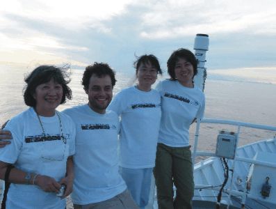 Figure 9. From left to right: Silvia
Watanabe, Colomban de
Vargas, Hui Liu, and Yurika Ujiie, respectively from
Argentina, France, USA, and Switzerland.
Figure 9. From left to right: Silvia
Watanabe, Colomban de
Vargas, Hui Liu, and Yurika Ujiie, respectively from
Argentina, France, USA, and Switzerland.These unicellular pelagic organisms are particularly resilient to genetic analyses, in particular barcoding, due to their small size and divergent origins, very far from the better-known metazoans. In addition, the relative absence of morphological characters challenges classical taxonomy, and cryptic species appear to be widespread in these groups. The intense biomineralization of their skeletons plays a key role in sea-water chemistry and in the building of km-thick deep-sea sediments. If the large majority of oceanic plankton is remineralized in the water column, the skeletonized microplankton have left in the geological record by far the most complete and well preserved fossil archive, so that a better assessment of species diversity and ecology will allow further understanding of how plankton and paleo-oceans have co-evolved.
Skeletonized microzooplankton were immediately isolated from the fresh, living samples into Petri-dishes. Cells were individually picked under the dissecting microscope using brushes, and sub-sampled, species by species, into smaller plastic dishes filled with filtered sea-water. The samples were then carefully examined, and representative specimens were photographed before being isolated into a special DNA-extraction buffer that preserves both nucleic acids and carbonate skeletons (GITC, de Vargas et al., unpublished).
In total, 1541 single-cell DNA extractions were realized along the 5 main stations (see Appendix 3 for complete listing). Nineteen morphological species of planktonic foraminifera were observed (Candeina nitida, Globigerina humilis, Globigerinella aequilateralis, Globigerinita glutinata, Globigerinoides conglobatus, Globigerinoides rubber, Globigerinoides sacculifer, Globorotalia crassaformis, Globorotalia hirsute, Globorotalia inflata, Globorotalia menardii, Globorotalia truncatulinoides, Globorotalia tumida, Hastigerina digitata, Hastigerina pelagica, Neogloboquadrina dutertrei, Orbulina universa, Pulleniatina obliquiloculata, Pulleniatina finalis), which represent about half the known, morphologically defined living “species”. In addition, 892 pictures of living specimens were taken before DNA extraction in order to document the morphological aspects – color, texture, etc.– of living cells (Figure 10) , which is a first in foraminifera research.
Species diversity and abundance varied significantly between the 5 stations (Figure 11). The populations were rich, abundant, and contained large adult specimens at Station 1, while much smaller and rare cells were observed at the following stations. This is probably linked to the moon cycle. Most species of foraminifera – mainly those living in shallow water – reproduce at or close to the full moon, which occurred in the evening of April 13th at our Station 1.
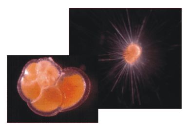 Figure 10. The spinose
species Globigerinoides sacculifer
and the non-spinose taxon Globorotalia menardii.
Characters such as color and spines are not preserved
after the death of the cell, but maybe significant for
taxonomy. (Photos by C. de Vargas)
Figure 10. The spinose
species Globigerinoides sacculifer
and the non-spinose taxon Globorotalia menardii.
Characters such as color and spines are not preserved
after the death of the cell, but maybe significant for
taxonomy. (Photos by C. de Vargas)Details of morphospecies distribution are not shown in this short final report. However, at each station, a clear depth zonation was revealed thanks to the stratified sampling. An example is given in Figure 12, which shows the number of DNA extractions performed for each MOCNESS-Net (1 to 8, from the deepest to the shallowest). Physical parameters of the water column, measured in real-time by the MOCNESS, are shown on the left part of the Figure 12. We note the presence of unique morphospecies in deep layers below the Deep Chlorophyll Maximum (DCM, ~50m), such as G. truncatulinoides or G. hirsuta. Species diversity increases toward surface waters, with a peak right within the DCM. The details of morphospecies distribution with depth will be studied by Sylvia Watanabe, using the archive samples preserved in ethanol or formalin.

Figure 11. Number of DNA extractions
realized per species and at each station. Note
that all
graphs are on the same scale, except for Station 2 where abundance was very low.
Future genetic analyses will allow us to solve the biological meaning of interesting morphological and ecological patterns we observe at the morphospecies level. For instance, we detected a clear change in the coiling direction of the shells of Globorotalia truncatulinoides between Stations 1 and 3 (Left from Right coiling shells, Figure 13A.)
The change in coiling direction in Globorotalia truncatulinoides is a classic in Micropaleontology and has been related to glacial-interglacial cycles. In our cruise, we observed this change not only between stations but also within depths at the same station (Figure 13B, data by S. Watanabe). Our data confirm that the Left-coiling truncatulinoides prefers cooler water, both in horizontal and vertical dimensions of the oceans, and genetic data will tell us if this morphologic change is associated with speciation.
Figure 12. Number of single-cell
specimens used for DNA extraction collected by depth
at Station 1.
Besides foraminifera, our team worked on two other groups of giant protists building elaborate skeletons: the radiolarians and coccolithophores. During most dives, Larry Madin and Erich Horgan collected wonderfully preserved colonial radiolarians. Detailed photographs of the colonies, individual cells and their symbionts were taken, and pieces of single colonies were preserved for DNA (frozen) and morphological (formalin and ethanol) analyses (Appendix 4).
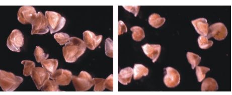 Figure 13A. Populations
of Left-coiling and Right-coiling G.
truncatulinoids, respectively, from stations 1 and 3. (Photo by C. de
Vargas).
Figure 13A. Populations
of Left-coiling and Right-coiling G.
truncatulinoids, respectively, from stations 1 and 3. (Photo by C. de
Vargas).Finally, an intense effort to collect coccolithophores was done by Hui Liu, graduate student at Rutgers University, as described next.
Hui Liu addition:
 Figure 13B. Ratio of
Left (green)/Right (yellow) coiling shells in the population of G. truncatulinoides sampled at Station 3. Data
were obtained by Silvia Watanabe using the formalin preserved fraction.
Figure 13B. Ratio of
Left (green)/Right (yellow) coiling shells in the population of G. truncatulinoides sampled at Station 3. Data
were obtained by Silvia Watanabe using the formalin preserved fraction.“It is really a great experience and rare opportunity for me to be here. The twenty days of intense working, learning, and enjoying the deep blue not only advanced my knowledge and skills in exploring the mystery of marine life, but also transformed my vision of research and life.
Other than helping with the MOCNESS sample processing, and sorting foraminifera once in a while, my major job during the CMarZ cruise was to collect coccolithophore samples for biodiversity and biogeography studies of key coccolithophore taxa, using a combination of genetic, molecular, and morphological analyses. Sea water was collected at each station from different depths using a bucket (surface), Niskin bottles (within the DCM and in intermediate waters within the mixed layer) and phytoplankton nets with 5 or 10 µm mesh size (~15 m depth). The water sample was transferred immediately to the main lab and filtered through 5 different types of membranes: Poly-Ether Sulphone for total DNA extraction, Polycarbonate for Scanning Electron Microscopy (SEM) , Cellulose nitrate for optic Microscopy, and ANODISC and AAWP for Fluorescent In Situ Hybridization (FISH). Altogether 750 liters of water were filtered and 121 filters were obtained. Ten out of twenty-nine DNA samples were selected to perform DNA extraction on board using the DNeasy plant mini kit. Large Subunit (LSU) ribosomal DNA was then amplified using the Polymerase Chain Reaction (PCR) method with primers specific to the Haptophyta (coccolithophores): Hapto4 and Leuk34r. The amplified DNA will be further used for a clone library and DNA sequencing analyses after the cruise. Optic microscopy, SEM and FISH samples will be analyzed as well to identify the boundaries between species and life cycle stages at different depths. In addition, basic cruise track data (salinity, temperature, fluorometry, pCO2, etc.) will be needed to characterize the water-masses and hydrography of the samples’ locations.
The cruise is ending soon. I’m very happy to get nice samples for my future work and I’ve learned a great deal. I’d like to thank everyone who worked together as a team and made everything possible, who patiently taught me how to collect and process the MOCNESS samples, who introduced different groups of zooplankton and techniques which I’m not familiar with, who helped me with collecting hundreds of liters of water, who kindly built the filtration holder for me, who generously loaned me whatever I asked for, and who made jokes and good coffee when I got tired. Finally, I want to say to Martin, ‘You are the inspiration of all of us’.”
14.0 Microzooplankton – Tintinnids (Barbara Costas)
The objective was to sample the epipelagic and if possible mesopelagic regions of the tropical/subtropical waters west of the mid-Atlantic ridge to collect and identify tintinnids. This includes both traditional identification through preservation with Lugol’s Iodine Solution (Acetic), “Lugal’s”, as well as amplification of the internal transcribed spacer region (ITS) of the rDNA gene and potentially the COI region as well.
Two basic approaches to sampling were used for the collection and identification of tintinnids. The first sampling approach involved collection of bulk water from two depths via a 30L Niskin bottle. The second sampling approach involved examining samples collected in the smaller nets (1/4-m MOCNESS, Reeve net, and various hand-deployed Ring nets) and picking out individual tintinnids for identification and DNA sequencing. Table 9 contains the details of the various sampling activities at the stations.
14.2.1 Bulk Water Sampling: A total of 60L of water was used per depth, so water was combined from two casts. From this water a sample (500ml) was taken for later chlorophyll a and pigment analysis (via High Profile Liquid Chromatography, or HPCL) by filtering onto a borosilicate glass fiber filter and preserving at -80̊C. A 500 ml sample of water was preserved with Lugol’s to a final concentration of 5%. This water will be examined via microscopy back at the University of Connecticut’s Department of Marine Sciences (UCONN DMS) for identification and enumeration of the tintinnids to at least genus level. Any naked ciliates will also be enumerated and identified where possible. The water was then concentrated gently via reverse filtration using a 20 µm sieve. The concentrated water was then separated into 5 aliquots (1/2, 1/6th [two replicates], and 1/18th [two replicates] of the concentrate volume) and filtered onto 3.0 µm cellulose nitrate filters. These filters were placed into 1.5 ml tubes and stabilized with a DNA prep buffer. Upon returning to UCONN DMS, the DNA will be extracted from the filters and primers specific to the Phylum Ciliophora and Class Spirotrichea will be used to amplify the ITS region. Libraries of the ciliates present at the various depths and locations will then be created allowing for comparison between depths and stations.
Table 9. Sampling activities associated with Tintinnid identification during the cruise. The table contains the cruise event number, station and cast information, and sampling activities and depth.
| Event Number | Station | Cast | Sampling Activity | Depth |
| RB10306.004 | 1 | 2 | 10µm Hand Ring Net | 10m |
| RB10406.004 | 1 | 1 | Niskin bottles | 10m & 75m |
| RB10406.008 | 1 | 2 | ¼-m MOCNESS | 500-350m, 350-200m, 200-150m, 150-100m, 100-75m, 75-50m, 50-25m, and 25-0m |
| RB10406.010 | 1 | 2 | Reeve Net | 500m |
| RB10606.003 | 2 | 2 | Niskin bottles | 15m & 75m |
| RB10606.005 | 2 | 3 | Reeve Net | 500m |
| RB10906.002 | 3 | 5 | Reeve Net | 200m |
| RB10906.009 | 3 | 3 | Niskin bottles | 15m & 75m |
| RB10906.016 | 3 | 2 | 10µm Hand Ring Net | 10m |
| RB11306.002 | 4 | 7 | Reeve Net | 200m |
| RB11306.007 | 4 | 2 | 5µm Hand Ring Net | 15m |
| RB11306.011 | 4 | 5 | 64µm Hand Ring Net | Surface |
| RB11306.016 | 4 | 4 | Niskin bottles | 45m & 100m |
| RB11306.014 | 4 | 8 | Reeve Net | 200m |
| RB11506.003 | 5 | 9 | Reeve Net | 200m |
| RB11506.014 | 5 | 5 | Niskin bottles | 40m & 100m |
| RB11506.012 | 5 | 10 | Reeve Net | 200m |
| RB11706.006 | 5 | 6 | ¼-m MOCNESS | 350-230m, 230-170m, 170-150m, 150-120m, 120-110m, 110-90m, 90-70m, 70-0m |
| RB11706.008 | 12 | 5 | Reeve Net | 200m |
14.2.2 Net Collection:
14.2.2.1 Quarter-meter MOCNESS nets: Where possible, a sub-sample of the ¼-m MOCNESS live fraction was examined for the presence of any swimming (live) tintinnids and/or loricas. A sampling of empty loricas was preserved in Lugol’s for further identification back at UCONN DMS. If any “live” animals (swimmers) were seen, they were pulled from the sub-sample, photographed, and set aside for DNA analysis through single cell PCR amplification and sequencing of the ITS region, and if possible COI. This work will be completed at UCONN DMS, although preliminarily analysis of preserved loricas was conducted during the cruise. Table 10 contains preliminary identification data based on the lorica analysis.
Table 10. List of ciliates found in the various net casts examined. The event number matches the cruise event log and Table 9. Tintinnid designation was the preliminary number given to tintinnids (or nakeds) based on lorica shape and size as well as swimming behavior (live). Please refer to Appendix 5 for images and preliminary identification of the tintinnids listed. The comment column describes how the tintinnid (or naked) was processed.
| Event Number | Tintinnid Designation | Comments |
| RB10306.004 | Tin 1 | Individual single cells picked from ½ of sample. Also digital images and Lugol’s preserved sample. |
| Tin 2 | Individual single cells picked from ½ of sample. Also digital images and Lugol’s preserved sample | |
| Tin 3 | Individual single cells picked from ½ of sample. Lugol’s preserved sample. | |
| RB10406.008 | ||
| 1. Net 1 | Tin 2 and Tin 8 | Lugol’s preserved sample (no lives) |
| 2. Net 2 | Tin 2, 3, 5, and 6 | Lugol’s preserved sample (no lives) |
| 3. Net 3 | Tin 2, 3, 5, 6, and 8 | Lugol’s preserved sample (no lives) |
| 4. Net 4 | Tin 2, 3, 5, 6, and 8 | Lugol’s preserved sample (no lives) |
| 5. Net 5 | Tin 2, 2a, 3, 6 | Lugol’s preserved sample (no lives) |
| 6. Net 6 | Tin 2, 2a | Lugol’s preserved sample (no lives) |
| 7. Net 7 | No loricas observed | Lugol’s preserved sample (no lives) |
| 8. Net 8 | Tin 3 and 6 | Lugol’s preserved sample (no lives) |
| RB10406.010 | Tin 2 | Individual single cells picked from sample. Lugol’s preserved sample. |
| Tin 5 | Individual single cells picked from. Also digital images and Lugol’s preserved sample. | |
| Tin 6 | Individual single cells picked from. Also digital images and Lugol’s preserved sample. | |
| Tin 7 | Individual single cells picked from sample. Lugol’s preserved sample. No picture | |
| Tin 8 | Individual single cells picked from sample. Lugol’s preserved sample. No picture | |
| RB10606.005 | Tin 8 | Individual single cells picked. Individuals placed into DNA buffer (bulk). Picture and Lugol’s preserved. |
| Tin 2 | Individual single cells picked. Individuals placed into DNA buffer (bulk). Picture and Lugol’s preserved. | |
| Tin 2a | Individual single cells picked. Individuals placed into DNA buffer (bulk). Picture and Lugol’s preserved. | |
| Tin 9 | Individual single cells picked. Individuals placed into DNA buffer (bulk). Picture and Lugol’s preserved. | |
| Tin 6 | Individual single cells picked. Individuals placed into DNA buffer (bulk). Picture and Lugol’s preserved. | |
| Tin 5 | Individual single cells picked. Individuals placed into DNA buffer (bulk). Picture and Lugol’s preserved. | |
| Tin 10 | Individual single cells picked. Individuals placed into DNA buffer (bulk). Picture of live. | |
| RB10906.002 | Tin 11 | Individual single cells picked. Individuals placed into DNA buffer (bulk). Picture and Lugol’s preserved. |
| Tin 2 | Individuals placed into DNA buffer | |
| Tin 12 | Individual single cells picked. Picture of live. | |
| Tin 13 | Individual single cells picked. Individuals placed into DNA buffer (bulk). Picture and Lugol’s preserved. | |
| Tin 14 | Individual single cells picked. Individuals placed into DNA buffer (bulk). Picture and Lugol’s preserved. | |
| Tin 6 | Individuals placed into DNA buffer | |
| Tin 5 | Individual single cells picked | |
| RB10906.016 | Tin 11 | Few, but picked individuals and placed into DNA buffer |
| RB11306.002 | Tin 2 | Individual single cells picked. Individuals placed into DNA buffer (bulk). Picture and Lugol’s preserved. |
| Tin 11 | Individual single cells picked. Individuals placed into DNA buffer (bulk). Picture and Lugol’s preserved | |
| Tin 15 | Individual single cells picked. Individuals placed into DNA buffer (bulk). Picture and Lugol’s preserved | |
| Tin 16 | Individual single cells picked. Individuals placed into DNA buffer (bulk). Picture and Lugol’s preserved | |
| Tin 17 | Individual single cells picked. Individuals placed into DNA buffer (bulk). Picture and Lugol’s preserved | |
| Tin 18 | Individual single cells picked. Individuals placed into DNA buffer (bulk). Picture and Lugol’s preserved | |
| Tin 9 | Individual single cells picked. Picture and Lugol’s preserved. | |
| Tin 19 | Individual single cells picked. Picture and Lugol’s preserved. | |
| Tin 2a | Individual single cells picked | |
| Tin 5 | Individual single cells picked. Individuals placed into DNA buffer (bulk). | |
| Tin 14 | Individuals placed into DNA buffer. | |
| Tin 20 | Individual single cells picked. Picture and Lugol’s preserved | |
| Tin 8 | Saw empty loricas | |
| RB11306.007 | Naked A | Individual single cells picked. Picture and Lugol’s preserved |
| Naked B | Picture and Lugol’s preserved | |
| Naked C | Picture and Lugol’s preserved | |
| Tin 19 | Individual single cells picked | |
| RB11306.011 | Tin 19 | Individual single cells picked |
| RB11306.014 | Tin 15 | Individuals placed into DNA buffer |
| Tin 17 | Individuals placed into DNA buffer | |
| Tin 19 | Individuals placed into DNA buffer | |
| Tin 14 | Individuals placed into DNA buffer | |
| Tin 5 | Individuals placed into DNA buffer | |
| Tin 16 | Individuals placed into DNA buffer | |
| Tin 2 | Individual single cells picked | |
| RB11506.003 | Tin 11 | Individual single cells picked. Picture and Lugol’s preserved. |
| Tin 16 | Individual single cells picked. Picture and Lugol’s preserved. | |
| Tin 19 | Individual single cells picked. Picture and Lugol’s preserved. | |
| Naked 21 | Individual single cells picked. Picture and Lugol’s preserved. | |
| Tin 15 | Individual single cells picked. Picture of live. | |
| Tin 22 | Individual single cells picked. Picture of live. | |
| Tin 17 | Individual single cells picked. Picture of live. | |
| Tin 5 | Individuals picked into DNA buffer | |
| Tin 8 | Saw empty loricas | |
| Tin 20 | Saw empty loricas | |
| RB11506.012 | Tin 16 | Individuals picked into DNA buffer |
| Tin 11 | Individuals picked into DNA buffer | |
| Tin 19 | Individuals picked into DNA buffer | |
| Tin 5 | Individuals picked into DNA buffer | |
| RB11706.006 | ||
| 1. Net 1 | No tintinnids seen (empty loricas or live) | |
| 2. Net 2 | No tintinnids seen (empty loricas or live) | |
| 3. Net 3 | Tin 20
Tin 17 Tin 22 |
Individual picked for single cell. Picture of live.
Also preserved empty loricas.
Preserved empty loricas (Lugol’s) Preserved empty loricas (Lugol’s) |
| 4. Net 4 | Tin 20
Tin 22 |
Preserved
empty loricas (Lugol’s)
Preserved empty loricas (Lugol’s) |
| 5. Net 5 | Tin 6
Tin 20 |
Individual picked for single cell. Picture of live.
Preserved empty loricas (Lugol’s) |
| 6. Net 6 | Tin 22 | Preserved empty loricas (Lugol’s) |
| 7. Net 7 | Tin 8
Tin 22 |
Preserved
empty loricas (Lugol’s)
Preserved empty loricas (Lugol’s) |
| 8. Net 8 | No tintinnids seen (empty loricas or live) | |
| RB11706.008 | ||
| Tin 19 | Individual single cells picked. Picture of live | |
| Tin 11 | Individual single cells picked. Picture of live. | |
| Tin 16 | Individual single cells picked. Picture of live. | |
| Tin 15 | Individual single cells picked. Picture of live. | |
| Tin 23 | Individual single cells picked. Picture of live. | |
| Tin 20 | Saw empty loricas. |
14.2.2.2. Sixty-four µm Reeve Net Tows: Water from Reeve Net tows was passed through a 150 µm mesh and then concentrated via gentle filtration with a 20 µm mesh. This concentrate was then examined for live tintinnids. Assumed similar species (based on general characteristics and swimming pattern) were then picked. Digital photos were taken, some were preserved with Lugol’s for further identification once back at UCONN DMS, and others set aside for DNA analysis through single cell PCR amplification and sequencing of the ITS region, and for many the COI as well. In addition, “same species” that seemed abundant were put into DNA prep buffer, which will allow extraction of the entire genome. Most single cell PCRs (Stations 1-4) were completed on-board the R/V Ron Brown. Station 5 and the actual sequencing analysis will be completed at UCONN DMS. Table 10 contains preliminary identification data based on lorica analysis.
14.2.2.3. Surface Ring Net Tows (5, 10, and 64 µm): Samples from several tows were examined for the presence of tintininds. Live tintinnids were picked, photographed, and, where possible, preserved in Lugol’s for further identification. Others of similar species were set aside for DNA (single cell) analysis. The PCR amplification for these samples was completed on the R/V Ron Brown, but sequence analysis of the ITS region and potentially the COI region will be completed at UCONN DMS. Table 10 contains any preliminary identification data based on lorica analysis. Note that the surface tows throughout the cruise had no or very few tintinnids, and therefore limited samples exist from these tows.
14.3 Discussion/Preliminary Observations
Little sampling of this region has previously been done in regards to the tintinnid community. Preliminary work has identified 22 potential tintinnid species and one potential naked ciliate species (“nakeds”). Appendix 5 contains images and preliminary identification where possible. Further examination of the preserved samples as well as finalizing the DNA analysis will clarify the number of species picked and identified. In addition, it is expected that examination of the preserved samples will provide for additional species, i.e. those smaller tintinnids that could not be properly captured in the relatively large-mesh nets (64 µm).
The cruise produced ten community DNA samples (two depths at each station) and ten corresponding preserved water samples from the bulk water sampling. In addition, there are Lugol’s preserved water samples from the various Reeve Net tows examined as well as individual loricas preserved from the these and other net samples (see Table 9). Over 500 tintinnids were picked for single cell DNA analysis (this includes multiples from assumed similar species), as well as an additional 400 animals placed into DNA prep buffer for bulk extraction of potentially 12 preliminarily identified species.
Prior to the cruise, we would have expected to find the tintinnids in the upper water column, i.e. near the phytoplankton (their expected food source). Examination of the samples from the various surface (to 15 m) ring net tows indicates that, at least at the five stations sampled, the tintinnid community is generally below 15 m. The two ¼-m MOCNESS tow samples that were examined for tintinnids (the only net system capable of capture), indicates that the tintinnid biomass is quite deep in the water column, and in the case of the MOC-¼ cast 2, down to 500m. In fact, in both MOC-¼ casts 2 and 6 no tintinnid loricas (or swimmers) were found to be in the samples from the top net (surface waters).
The overall diversity of the tintinnids based on the preliminary work and identification indicates the most species at Stations 4 and 5. There is also the potential that several of the same species were present throughout much of the sampling region, including one at Stations 1 through 4 and two at Stations 2 through 5. (See Table 10 and Figure 14). Preliminary work does not indicate that any one species was present at all 5 stations; however, the analysis of the bulk water DNA may show otherwise.
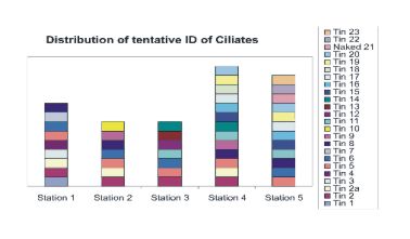 Figure 14. Distribution
of tentative species found by
station. Blocks are only representative of
presence/absence, not abundance. Station 4 had the most
diversity followed by Station 3. Several tentative species
were found at multiple stations.
Figure 14. Distribution
of tentative species found by
station. Blocks are only representative of
presence/absence, not abundance. Station 4 had the most
diversity followed by Station 3. Several tentative species
were found at multiple stations.
15.0 Pelagic fishes (Tracey Sutton)
The large-gear bathypelagic sampling conducted during the 2006 CMarZ cruise aboard the NOAA research vessel Ron Brown provided a unique opportunity to sample and census deep-pelagic fishes that are often missed by standard trawling procedures (i.e., smaller, but more numerous forms that pass through the mesh of fisheries-style trawling gear). The combination of discrete depth sampling via the MOCNESS, fine-mesh nets designed and constructed specifically for this endeavor, and an experienced operating crew has generated a valuable and quantitative collection of specimens from the poorly known bathypelagic realm. A brief summary of quantitative methods and preliminary results are provided below.
The primary collecting gear for deep-pelagic fishes were the 1-m and 10-m MOCNESS midwater trawls, outfitted with 333-μm mesh nets (excepting the initial oblique deployment net of 3-mm mesh). Immediately following gear retrieval and sample wash-down, all fish specimens were sorted from the catch and processed completely in a systematic fashion. All specimens were identified, measured to the nearest 0.1 mm (standard length) and enumerated. Biomass (g wet weight) was estimated for all specimens using taxon-specific length/weight regressions. Abundance and biomass data were then pooled for each net sample, tow, and station to gain a quantitative view of fish assemblage structure, both in terms of biodiversity and relative composition. Tissue samples were taken of selected species for DNA-barcoding analyses.
15.2.1 Assemblage Structure. A total of 3,965 fish specimens were collected, representing minimally 127 species (84 genera), from 42 families. The high ratio of genera and families to total species number is often a truer measure of diversity than species counts per se, as high counts of the latter are often the result of taxonomic ‘splitting’ of certain focus groups. A complete species list, with raw abundances (not normalized for volume filtered) by station is presented in Appendix 7. Two things were readily apparent from initial scan of these data: 1) we did not approach an asymptote for species versus effort, as reflected by the high numbers of new species in later trawls; 2) excepting the numerical dominance of the genus Cyclothone (68% of all specimens), diversity as a function of species number per total specimen abundance was quite high – roughly two out of three bathypelagic species were represented by less than five specimens.
As expected for low-latitude bathypelagic ecosystems far removed from topographic features (i.e. ridges, canyons), fish biomass was quite low. The entire fish catch from the cruise amounted to just under 500 g wet weight biomass. As with abundance, the genus Cyclothone dominated the biomass of the assemblage, but to a lesser degree than with numbers, since the biomass contribution by large dragonfishes (e.g. Rhadinesthes, Eustomias, Photonectes) was quite significant.
Integration of current knowledge on species’ vertical distributions with catch data from this cruise suggests some degree of contamination from shallower depth strata, particularly from mesopelagic myctophid species (Diaphus, Lepidophanes), but this amount was not major compared to the taxa that we caught that are considered truly bathypelagic. These taxa include the ceratioid anglerfishes (8 species from 5 families), the bathypelagic eels (Eurypharynx, Saccopharynx, and Serrivomer), the great swallowers (Chiasmodon and Pseudoscopelus), and the whalefishes (Cetostoma and Rondeletia). Perhaps the best indicator of the discreteness of the bathypelagic sampling in these waters was what we didn’t get – the upper mesopelagic zone here is generally dominated by myctophids (Diaphus, Notolychnus, Myctophum) and lightfishes (Vinciguerria and Pollichthys) and shallow hatchetfishes (Maurolicus, Valencienellus). These represented a minor component of abundance and biomass, but did add to the species richness total. A brief foray into the mesopelagic zone during the last MOC10 deployment (MOC-10-07-Net 4) showed fairly conclusively that the low catches we had observed in the deep tows were a true measure of the low biomass at depth rather than a flaw in the fishing ability of the new MOCNESS configuration. Indeed, nearly 1,000 specimens were taken in this net, including some very large myctophid and dragonfish specimens. This sample would be considered a large haul with standard midwater trawls (i.e. Tucker trawl with 3-mm mesh).
15.2.2 Rare species: One of the most exciting features of bathypelagic trawling is that every tow potentially contains undescribed or very rare species. Some of the notable catches from this cruise were:
● 5 species of the genus Eustomias (most cruises usually generate only one or two specimens); this genus is an ideal target for addressing the oceanic species concept. There are presently 115 described species in this genus, all separated by a single character (barbel form). Tissue was taken from all for barcoding, which may help unlock this mystery.
● Male anglerfishes from 5 families were taken. The taxonomy of male ceratioids is so poorly known due to their rarity and undersampling, keys do not exist for most species. As with Eustomias, fish tissue was taken from all to match them with keys for females, thus enabling the construction of a key for the most speciose bathypelagic fish group.
● Leptostomias sp. nov. (1 specimen): this is one of the most well-defined genera of dragonfishes, all of which I am quite familiar with. All described species have a barbel at least 50% of their body length (this specimen is 10%) that terminates in a simple bulb with either one or two filaments. This specimen has a barbel with well-developed tentacles (> 12 in number), each of which is innervated and vascularized.
● Pseudoscopelus “sp. A” cf. obtusifrons (1 specimen): this specimen varies from its nearest neighbor (P. obtusifrons) in the pattern of photophores and the form of the premaxillary teeth, both of which are diagnostic characters for the genus.
● Astronesthes cf. indicus (1 specimen): I am quite familiar with this tropical species, and the specimen that we took was shorter (lower photophore counts) and had a longer barbel than the classic form of the species.
16.0 Larval Fish (C.B. Lalithambike Devi)
The zooplankton collected using MOC1 and MOC10 were analyzed in the ship's lab immediately after each tow. The fish larvae were picked live from the whole sample and were kept in the cold room for further analysis. The subsampled zooplankton preserved in ethanol and formaldehyde were also examined and the larvae picked out.
The fish larvae were identified into different taxa.
● 43 species belonging to 18 families were present in the live samples analyzed.
● The rest of the samples were preserved in formaldehyde for further studies after the cruise.
● Maximum abundance and diversity(4 families and 7 species) were observed at lat 29o 57'N and lon 71o 01'W (MOC1 Tow 3 Net 5).
● Abundance and diversity decreased from there. Only 2 families with 7 species were found at 25o 00'N and 59o 56'W (taken from 0-1000m).
● At lat 33o 38'N and lon 69o 47'W, 5 species were encountered in 4 families (MOC10 Tow 1 Net 4).
● In all the three locations, the mesopelagic groups Myctophidae and Gonostomatidae were dominant.
● Two of the Cyclothone species (C. braueri and C. pallida) contributed the most to the numerical abundance.
● Maximum species diversity was observed in the family Myctophidae (15 species).
● Notoscopelus resplendens and Benthosema glaciale were the dominant species found in the area.
● Thunnus sp. was found only in one sample (MOC10 Tow5 Net 4) at 19o 49'N and 54o 44'W.
● The members of the Percoids were rare.
● 15 species were given for barcoding.
The lanternfish family Myctophidae is the most widespread family of midwater fish in the world ocean. Their larvae are highly prominent in the open ocean plankton samples.
17.0 Team DNA Sequencing (Rob Jennings, Paola Batta Lona, Brian Ortman, Ebru Unal, Leo Blanco Bercial)
The molecular group had an extremely successful cruise. We assembled our fully functional lab before the ship left port, and were already running test PCRs and sequencing reactions while underway to the first station. After an initial burst of sequencing of some of the samples from Stations Zero and One, the team had to develop a modified sequencing reaction cleanup protocol. We discovered that the high humidity and salty air were causing precipitation in our ethanol and EDTA solutions. Upon fixing this problem, the sequencer ran trouble-free, and a lot of hard work reduced the backlog of samples to a large extent.
Combining Stations 0-5 (and including Station 3b), team DNA catalogued over 1200 individual organisms, comprising 523 species from 12 phyla (Table 11). Of these, we extracted DNA from about 770 individuals, and were successful in PCR amplifying roughly 80% of these individuals. Complete, edited barcodes (requiring good sequence reads in both directions) were obtained for about 100 species, and processing is still ongoing for another 100 species. Given our goal of sequencing three individuals per species, the ~200 COI barcodes obtained in barco reflect a sequencing effort of many hundred reactions. This level of output reflects the hard work and perseverance of the entire DNA team and represents perhaps an order of magnitude higher throughput than most land-based labs of our type and size typically yield.
Table 11. Species collected and submitted for sequencing and individuals with DNA extracted.
| Taxonomic group | # Species Collected | # Individuals Extracted | |
| Arthropods | |||
| Amphipoda | 31 | 47 | |
| Copepoda | 138 | 190 | |
| Mysidacea | 6 | ||
| Other Crustacea | 18 | 23 | |
| Euphausiidae | 14 | 20 | |
| Ostracoda | 58 | 100 | |
| Cnidaria | |||
| Anthozoa | 1 | 0 | |
| Hydrozoa | 103 | 166 | |
| Scyphozoa | 7 | 12 | |
| Mollusca | |||
| Gastropoda | 50 | 107 | |
| Other Mollusca | 27 | 17 | |
| Others | |||
| Cephalochordata | 1 | 2 | |
| Chaetognatha | 1 | 1 | |
| Ctenophora | 22 | 31 | |
| Echinodermata | 1 | 1 | |
| Larvacea | 12 | 26 | |
| Nemertea | 1 | 3 | |
| Polychaeta | 3 | 4 | |
| Thaliacea | 14 | 18 | |
| Pisces (larval) | 15 | ||
| Total | 523 | 768 | |
Team DNA did not get to as much on-board analysis and comparison of the DNA barcodes we generated as we might have liked. Nevertheless, many engaging conversations with the taxonomists have left us with intriguing molecular puzzles to pursue. Some of these questions reflect ongoing or proposed projects, while others came up de novo as we worked. These lines of research can be partly answered once we finish analyzing the barcodes already collected; full answers may require more samples and sequencing. Some of these questions involve using bulk extraction and cloning of amplified DNA to identify prey items in the guts of several species (we have gut samples from fish suspected of eating siphonophores, as well as from siphonophores suspected of eating fish). Others involve sequencing two alternate forms of what has to date been described as a single species (e.g., a “large” and “small” form, or a form with colored spots and a form without spots) to see if they truly belong to the same species. In many instances, connecting the taxonomic question to the molecular methodologies required to answer it might never have happened (or at least taken much longer to arise) if not for the presence of both kinds of experts on this cruise.
Apart from initiating research questions, the sequences collected on this cruise are a tremendously valuable addition to the catalogue of DNA barcodes for marine zooplankton, particularly in the under-sampled deep waters trawled on this cruise. As stated by others, although overall biomass was low in these deep layers, species diversity was quite high, allowing us to obtain DNA barcodes for a vast array of species. Our collections include many of the same species from different stations, which will enable us to investigate the spatial scale of genetic cohesiveness in the future. Although many zooplankton species are usually thought to have huge abundances and effective population sizes, the various regimes we moved through over the course of our cruise track (subtropical, Sargasso, tropical, etc.) could possibly create barriers to gene flow that might reveal themselves as we analyze our samples more fully.
18.0 Silhouette photography, CMarz web site (Nancy Copley and Dicky Allison)
18.1 Silhouette Photography (N. Copley)
Silhouette photographs were taken of two MOC-1 night tows (8 nets each) , from stations 1 and 2 (MOC-01-002 and MOC-01-003) for later digital length and abundance analysis. In order to accomplish the photography, the ship’s salinity room was converted into a darkroom. This room proved adaptable, after a few modifications, due to its small size and double entry which excluded almost all light. The overhead lights had to be removed because there was no separate light circuit independent of the rest of the Hydo lab in the salinity room. Heavy black cloth was placed over both the inner and outer doors to keep out the light and duct tape was used to cover the internal lights of the Guildline Autosal which could not be turned off or moved. Following a seminar on using the WHOI Digitizer program which is used to measure and count zooplankton, the darkroom method of taking silhouette photographs was demonstrated to all those who were interested in seeing this technique.
In the wet lab, samples were split with a Motoda box splitter to a degree that allowed a sample to lie in a single layer (one specimen thick) in an 8" x 10" plexiglass box, typically between zero split and 1/16th split. In the darkroom, a sheet of photographic paper (Ilford multigrade IV RC Deluxe, 8" x 10") was labeled with tow, net and split information using a waterproof pen and placed in the box. A collar was inserted to hold the paper down and prevent plankton from slipping underneath, and then the sample was gently poured into the box. Timing the moment of exposure to the rocking of the ship was attempted so that the sample was not congregated on one side of the film but this was not always successful. A camera flash held about 3' above the sample was used to expose the film which was then developed using Kodak Polymax T developer (1-2 minutes), Stop Bath (10 seconds), and Rapid Fixer (3 minutes). The films were washed in a tray of circulating water for at least 10 minutes before rinsing with a dilute solution of Photo Flo to prevent spotting and hung to dry. Scanning the photographs and analyzing them will be done post-cruise.
18.2 CMarZ Web site (N. Copley and D. Allison)
A web site for the cruise was set up just prior to sailing and was maintained using ssh and ftp during the cruise. The url is www.cmarz.org/CMarZ_Cruise_April. “24/7" internet access had only recently become available at sea and we used it to the maximum extent possible on the Ron Brown. Both the Chief Scientist reports and the Teacher-at-Sea daily logs were posted. A photo gallery of the science party, of animals found in the samples, and of life on board the ship were also made available on these pages. Several short film clips were placed on the site: the dive boat being launched down the side of the Ron Brown, several types of gelatinous zooplankton swimming, the launching the three MOCNESS systems, an overview of how the samples were retrieved from the net and initially examined, and a view of the gene sequencer and associated computer output. Periodic updates to the cruise track were posted. A subdirectory was created for media outlets to download high resolution photographs and movie clips, www.cmarz.org/CMarZ_Cruise_April/images_press. These were accessed widely by print and internet sites worldwide.
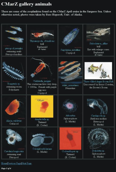
Figure 15. Page from the cruise website gallery of zooplankton showing a
variety of the zooplankton captured at sea.
19.0 Training on Zooplankton Sampling and Molecular Analysis (Chaolun Li)
As a researcher from the Institute of Oceanology, Chinese Academy of Sciences, and a member of CMarZ, I was pleased to participate in this CMarZ cruise funded by NOAA and to achieve my expected objectives.
Zooplankton sampling in the deep sea: A practicable and effective sampling method is essential to biodiversity study in the deep sea. With the advent of multiple opening-closing net systems in the mid-1900s, high-resolution sampling of the bathypelagic and abyssopelagic zones became possible. One of my objectives on this cruise was to become familiar with the MOCNESS, which was used to sample zooplankton throughout the water column. I received substantial training with the structure, working principles, and operation of the MOCNESS. I participated in the operation of the gear from the installation and loading of the nets to the setup and testing of the MOCNESS electronics. I also learned how to control the towing of the nets in realtime through the use of the deck unit and software controls and display.
Training of the molecular analysis of zooplankton: Shipboard molecular analysis of zooplankton was one of the most successful aspects of work on this cruise. Another of my objectives was to learn as much as possible about the molecular analysis of zooplankton. With the kindness and patience of the people in the DNA sequencing group, I experienced the whole process of COI analysis of zooplankton. Ebru Unal taught me about the process from DNA extraction and purification to PCR amplification. Rob Jennings showed me how to make a gel, do electrophoresis, and image analysis. This training will advance my skills in molecular analysis on zooplankton and help to unify the molecular approaches for zooplankton research ongoing at our institute in China. This will help to produce coordinated data from the China Sea and ensure its integration into the wider global database.
20.0 ARMADA Teacher at Sea Project (Joseph Catron)
As an ARMADA Teacher at Sea, I had the basic responsibility of participating in the CMarZ scientific endeavor in a capacity that would benefit the research process. In addition it was expected that I keep a journal of my experiences on the Ron H. Brown, and make these journals accessible via the Internet. Funding for my travel, and participation were provided by the ARMADA Project, through the University of Rhode Island. This program, in part, is designed to immerse science teachers in a real-world scientific investigation aboard NOAA ships. It is ARMADA’s expectation that these experiences will enrich the teacher, and in turn be shared with their colleagues and students. Beyond my basic requirements, I wanted to obtain a few practical ideas from the CMarZ project that I could develop into lesson plans, learn of career opportunities that my students may benefit from, remain in contact with my classroom, and gain a better appreciation for the ocean, which I teach about without having ever spent time at sea.
The basic expectations of my participation in the scientific process were met. Much of the scientific work in the CMarZ project required expertise in taxonomic identification of zooplankton. This skill is not easily transferable in a short amount of time. Therefore, I did not aid in this process, although I would have enjoyed learning to become proficient in identifying at least one major group of organisms. I did learn many specifics about the zooplankton that live in the pelagic oceans. The DNA barcoding lab was engaged in problem-solving and also under a tight schedule, so direct participation in their work was not possible. I did however get to spend time in the lab learning the process of DNA extraction, amplification, and sequencing. My direct support of the CMarZ project came from the help I provided in record keeping, launching and retrieving the MOCNESS systems, preserving specimens, and in general helping anywhere I was needed or could be used. I feel I was an asset to the CMarZ project in this respect.
While interacting with the participants on the CMarZ study, I was able to develop two lesson plan ideas, and I am working out the details of a third lesson. One lesson will involve students using silhouette photography, used by Nancy Copley at WHOI. I will have students use silhouettes to compare abundance, diversity, and biomass between the pelagic zones. Another lesson idea I developed was related to COI genes and microarrays. I penciled out a lesson that would teach students, in general, how a microarray chip can be used to test for species presence from a mixed DNA sample collected in a plankton tow. The third lesson is currently still in the planning stage. I would like to come up with a way to integrate the physics of light and pigments with the biology of bioluminescence of deep-sea organisms. Although these lessons are not in a final and ready-to-use format, I am pleased to have 3 relevant and creative lessons plan ideas.
The daily journal I was required to write, and post on the Internet worked well, thanks to Dicky Allison from WHOI. She was able to help edit my journal writing, and post my writings on the CMarZ Cruise Website. I was able to use this protocol to communicate with my students. My classes were covering animal taxonomy at the time, which was also occurring daily aboard the ship. I used many of the journal entries to introduce the students to different marine taxonomic groups. Each day, a question was posed to the students. They were asked to respond to me using email. This process was slow. I was slightly disappointed not to receive more answers in a timely fashion. This is primarily a reflection on not being able to communicate directly with my classroom. In general however, I feel the journaling and classroom connection was successful.
To address all of the things I have learned during this cruise would require a lengthy response. Having never been to sea, much of what I experienced was novel and each day was filled with a plethora of learning. One of the most important things I think my students will benefit from is what I learned about how important it is to be a scientifically literate person. During the cruise, press conferences occurred and reporters later printed what we were accomplishing on this project. In some instances, their reporting was grossly distorted. This provided me with a two-fold lesson. First, there is a need for the average person to be scientifically literate, and the other is that what appears in the general media about science may not always be accurate. All students should strive to become literate in science, as well as intelligently skeptical of what they read. I learned to better appreciate the great expanse of the ocean, as well as more details on its nature than I will include in this report. I am sure the next time we study the ocean in class, it will be with greater insight and detail. Finally, I have several career ideas to share with students when I return. These careers range from working as an engineer aboard a NOAA ship, to conducting scientific research at the Woods Hole Oceanographic Institution.
This cruise has been rewarding and enjoyable. All of my basic needs were well met, and my professional expectations were accomplished. I would like to thank Jill Johnen and Andrea Kecseks from the ARMADA Project for making this cruise possible. I am thankful to Ann Bucklin from AVERY Point, for helping me get set up to participate in the CMarZ project. I was disappointed that I did not get to meet her in person. I would like to give special thanks to Peter Wiebe, Nancy Copley, and Dicky Allison, from WHOI, for helping me find my niche, aiding me in meeting my goals, and for making this cruise a success.
| Science Party (Name, Institution ) | |
|---|---|
| Peter Wiebe (Chief Scientist) | Woods Hole Oceanographic Institution, USA |
| Dicky Allison | Woods Hole Oceanographic Institution, USA |
| Martin Angel | Nation al Oceanography Centre, UK |
| Leo Blanco Bercial | University of Oviedo, Spain |
| Joe Catron | Billings High School, Billings, Montana, USA |
| Nancy Copley | Woods Hole Oceanographic Institution, USA |
| Astrid Cornils | Alfred Wegener Institute, Germany |
| Barbara Costas | University of Connecticut, USA |
| Colomban de Vargas | Station Biologique, France |
| Lalithambika Devi | National Institute of Oceanography, India |
| Hege Øverbø Hansen | Institute of Marine Research, Norway |
| Russ Hopcroft | University of Alaska, USA |
| Erich Horgan | Woods Hole Oceanographic Institution, USA |
| Rob Jennings | University of Connecticut, USA |
| Mikiko Kuriyama | University of Tokyo, Japan |
| Chaolun Li | Institute of Oceanology, China |
| Dhugal Lindsay | JAMSTEC, Japan (& Australia) |
| Hui Liu | Rutgers University, USA |
| Paola Batta Lona | University of Connecticut, USA |
| Larry Madin | Woods Hole Oceanographic Institution, USA |
| Hiroyuki Matsuura | University of Tokyo, Japan |
| Brian Ortman | University of Connecticut, USA |
| Francesc Pagès | Institut de Ciències del Mar, Spain |
| Saramma Panampunnayil | National Institute of Oceanography, India |
| Tracey Sutton | Harbor Branch Oceanographic Institution, USA |
| Yurika Ujiie | University of Geneva, Switzerland |
| Ebru Unal | University of Connecticut, USA |
| Silvia Watanabe | Universidad de Buenos Aires, Argentina |
| Ship's Officers and Crew, R/V Ronald H. Brown | |
| Gary Petrae | Captain |
| Stacy Birk | Commander |
| Elizabeth Jones | Lieutenant |
| Jackie Almeida | Ensign |
| James Brinkley | Ensign |
| Priscilla Rodriguez | Lieutenant Commander U.S. Public Health Service |
| Frank Dunlop | Chief Engineer |
| Keegan Plaskon | 1st Assistant Engineer |
| Gordon Gardipe | 2nd Assistant Engineer |
| Wayne Smith | 3rd Assistant Engineer |
| Nick DiNicola | Wiper |
| Ben Zielke | Wiper |
| Bruce Cowden | Chief Bosun |
| David Owen | Bosun Group Leader |
| Reginald Williams | Deck Utilityman |
| Victoria Carpenter | Able Bodied Seaman |
| Phil Pokorski | Ordinary Seaman |
| Mary O'Connell | Ordinary Seaman |
| Jesse Byrd | Ordinary Seaman |
| Leo Wade | Ordinary Seaman |
| Richard Whitehead | Chief Steward |
| Karen Bailey | Chief Cook |
| Herb Watson | 2nd Cook |
| Michael Moats | General Vessel Assistant |
| Jonathan Shannahoff | Chief Survey Technician |
| Jeff Hill | Lead Electronics Technician |
APPENDIX 2. Summary of Blue Water Dive Collections.
APPENDIX 3. List of DNA extractions from foraminifera.
APPENDIX 4. Colonial radiolarians collected by diving that have had pieces preserved for DNA (frozen) and morphological (formalin and EtOH) analyses.
CMarZ (April 10-30th, 2006) |
|
|
|
|
|
|
||
Sample Name |
Sation |
Dive |
Lat |
Long |
Date |
Remark |
Formalin |
Etoh |
Rad1 |
3 |
3 |
24.84 |
-60.14 |
4/19/06 |
Night |
Y |
Y |
Rad2 |
3 |
3 |
24.84 |
-60.14 |
4/19/06 |
Night |
Y |
Y |
Rad3 |
3 |
3 |
24.84 |
-60.14 |
4/19/06 |
Night |
Y |
N |
Rad4 |
3 |
3 |
24.84 |
-60.14 |
4/19/06 |
Night |
Y |
N |
Rad5 |
3 |
4 |
24.98 |
-60.54 |
4/20/06 |
Day |
Y |
Y |
Rad6 |
3 |
4 |
24.98 |
-60.54 |
4/20/06 |
Day |
Y |
N |
Rad7 |
3 |
4 |
24.98 |
-60.54 |
4/20/06 |
Day |
Y |
N |
Rad8 |
3 |
4 |
24.98 |
-60.54 |
4/20/06 |
Day |
Y |
Y |
Rad9 |
3 |
4 |
24.98 |
-60.54 |
4/20/06 |
Day |
Y |
Y |
Rad10 |
3 |
4 |
24.98 |
-60.54 |
4/20/06 |
Day |
Y |
Y |
Rad11 |
3 |
4 |
24.98 |
-60.54 |
4/20/06 |
Day |
Y |
Y |
Rad13 |
3 |
5 |
24.96 |
-60.68 |
4/21/06 |
Day |
Y |
Y |
Rad14 |
3 |
5 |
24.96 |
-60.68 |
4/21/06 |
Day |
Y |
Y |
Rad15 |
3 |
5 |
24.96 |
-60.68 |
4/21/06 |
Day |
Y |
Y |
Rad16 |
3 |
5 |
24.96 |
-60.68 |
4/21/06 |
Day |
Y |
N |
Rad17 |
3 |
5 |
24.96 |
-60.68 |
4/21/06 |
Day |
Y |
Y |
Rad18 |
3 |
5 |
24.96 |
-60.68 |
4/21/06 |
Day |
Y |
Y |
Rad19 |
3 |
5 |
24.96 |
-60.68 |
4/21/06 |
Day |
Y |
Y |
Rad20 |
3 |
5 |
24.96 |
-60.68 |
4/21/06 |
Day |
Y |
Y |
Rad21 |
3 |
5 |
24.96 |
-60.68 |
4/21/06 |
Day |
Y |
N |
Rad22 |
3 |
5 |
24.96 |
-60.68 |
4/21/06 |
Day |
Y |
Y |
Rad23 |
3 |
5 |
24.96 |
-60.68 |
4/21/06 |
Day |
Y |
Y |
Rad27 |
4 |
6 |
19.82 |
-54.72 |
4/23/06 |
Day |
Y |
N |
Rad28 |
4 |
6 |
19.82 |
-54.72 |
4/23/06 |
Day |
Y |
Y |
Rad29 |
4 |
6 |
19.82 |
-54.72 |
4/23/06 |
Day |
Y |
Y |
Rad30 |
4 |
7 |
19.82 |
-54.47 |
4/24/06 |
Night |
Y |
Y |
Rad31 |
4 |
7 |
19.82 |
-54.47 |
4/24/06 |
Night |
Y |
Y |
Rad32 |
4 |
7 |
19.82 |
-54.47 |
4/24/06 |
Night |
N |
Y |
|
|
|
|
|
|
|
|
|
|
|
|
|
|
|
|
Total |
48 |
APPENDIX 5. Tintinnid images and designations followed by preliminary ID to family and genus if possible. Picture includes measurements of lorica length and lorica oral opening. Note: Non-live pictures are from Lugol’s preserved samples and color is not indicative of living tintinnid.
TIN 1
Preliminary ID – Famliy: Dictyocystidae, Genus: Dictocysta
TIN 2a
Preliminary ID – Family: Undellidae, Genus: Undella
TIN 2b
Preliminary ID – Family: Undellidae, Genus: Proplectella
TIN 3
Preliminary ID – Family: Cyttarocylidiae. Although ID is weak.
TIN 4 (No Figure)
Preliminary ID – This is probably same as TIN 2
TIN 5
Preliminary ID – Family: Codonellidae, Genus: Codennella
TIN 6
Preliminary ID – Family: Petalotrichidae?
TIN 7 (No Figure)
Preliminary ID – No ID yet. Need to look at preserved sample.
TIN 8
Preliminary ID – Family: Codonellopsidae, Genus: Codonellopsis
TIN 9
Preliminary ID – Family: Petalotrichidae, Genus: Petalotricha
TIN 10
Preliminary ID – No tentative ID yet
TIN 11
Preliminary ID – Family: Rhabdonellidae, Genus: Rhabdonella
TIN 12
Preliminary ID – Family: Xystonellidae, Genus: Xystonella
TIN 13
Preliminary ID – Family: Undellidae, Genus: Amplectella
TIN 14
Preliminary ID – Family: Xystonellidae, Genus: Xystoneliopsis
TIN 15
Preliminary ID – Family: Tintinnidae, Genus: Eutintinnus
TIN 16
Preliminary ID – Family: Rhabdonellidae, Genus: Rhabdonella
TIN 17
Preliminary ID – Family: Xystonellidae, Genus: Xystonella
TIN 18
Preliminary ID – Family: Rhabdonellidae, Genus: Rhabdonella
TIN 19
Preliminary ID – No preliminary ID yet
TIN 20
Prelilminary ID – No preliminary ID yet
NAKED 21
Preliminary ID – No preliminary ID yet
TIN 22
Preliminary ID – No preliminary ID yet
TIN 23 (No Figure)
Preliminary ID – No preliminary ID
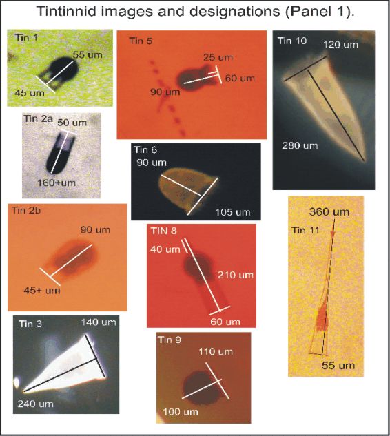

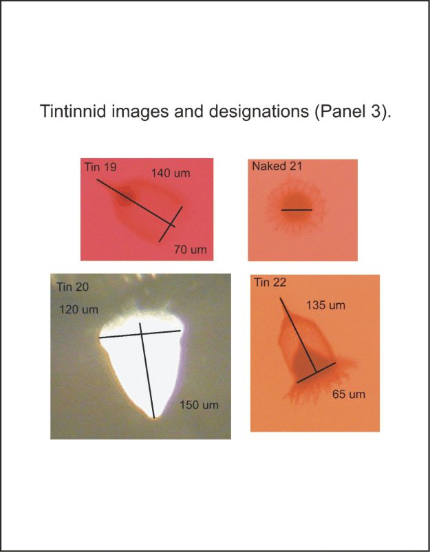
APPENDIX 6. MOCNESS Deployment Log. Summary of 1-m, 10-m and 1/4-m MOCNESS Tows (local Date/Time).
|
Station 1 |
Station 2 |
Station 3 |
Station 4 |
Station 5 |
Cruise |
Species |
Totals |
Totals |
Totals |
Totals |
Totals |
Totals |
Argyropelecus aculeatus |
2 |
15 |
0 |
2 |
6 |
25 |
Argyropelecus gigas |
0 |
0 |
0 |
0 |
5 |
5 |
Argyropelecus hemigymnus |
2 |
12 |
10 |
11 |
13 |
48 |
Argyropelecus larva |
0 |
0 |
2 |
1 |
4 |
7 |
Ariosomma leptocephalus |
0 |
0 |
0 |
1 |
0 |
1 |
Aristostomias xenostoma |
0 |
0 |
0 |
0 |
1 |
1 |
Astronesthes cf indicus |
0 |
0 |
0 |
0 |
1 |
1 |
Astronesthes juvenile |
0 |
0 |
0 |
0 |
2 |
2 |
Astronesthes micropogon |
0 |
0 |
0 |
0 |
1 |
1 |
Astronesthes similis |
0 |
0 |
0 |
0 |
1 |
1 |
Avocettina infans |
0 |
2 |
0 |
0 |
0 |
2 |
bathylagid larva |
0 |
0 |
0 |
0 |
0 |
0 |
Benthalbella infans |
0 |
0 |
1 |
0 |
0 |
1 |
Benthosema suborbitale |
0 |
2 |
0 |
0 |
8 |
10 |
Bolinichthys indicus |
1 |
0 |
0 |
0 |
0 |
1 |
Bolinichthys juvenile |
0 |
0 |
0 |
0 |
3 |
3 |
Bolinichthys photothorax |
0 |
2 |
1 |
1 |
7 |
11 |
Bonapartia pedaliota |
0 |
3 |
1 |
1 |
1 |
6 |
Bothid larva |
2 |
0 |
10 |
0 |
11 |
23 |
Brama caribbea |
0 |
0 |
0 |
0 |
1 |
1 |
Bregmaceros atlanticus |
0 |
0 |
1 |
2 |
8 |
11 |
Ceratias holboelli |
0 |
0 |
0 |
0 |
1 |
1 |
Ceratiid male |
0 |
0 |
1 |
0 |
0 |
1 |
Ceratioid larva |
0 |
0 |
0 |
1 |
0 |
1 |
Ceratoscopelus warmingii |
1 |
1 |
10 |
9 |
31 |
52 |
Cetostoma regani |
0 |
0 |
1 |
0 |
0 |
1 |
Chauliodus danae |
0 |
2 |
4 |
2 |
0 |
8 |
Chauliodus sloani |
1 |
3 |
0 |
1 |
0 |
5 |
Chiasmodon niger |
1 |
0 |
0 |
0 |
0 |
1 |
Coccorella atlantica |
0 |
1 |
0 |
0 |
0 |
1 |
Coryphaena hippurus |
0 |
0 |
1 |
0 |
0 |
1 |
Cryptopsaras couesii |
0 |
2 |
0 |
0 |
0 |
2 |
Cyclothone acclinidens |
0 |
0 |
0 |
7 |
165 |
172 |
Cyclothone alba |
0 |
0 |
1 |
2 |
0 |
3 |
Cyclothone braueri |
138 |
412 |
214 |
142 |
367 |
1273 |
Cyclothone microdon |
131 |
99 |
45 |
41 |
64 |
380 |
Cyclothone pallida |
217 |
83 |
181 |
66 |
383 |
930 |
Cyclothone pseudopallida |
18 |
52 |
1 |
0 |
23 |
94 |
Cyclothone (damaged) |
1 |
0 |
1 |
1 |
0 |
3 |
Cyclothone larvae |
0 |
10 |
0 |
0 |
0 |
10 |
Diaphus brachycephalus |
0 |
0 |
1 |
1 |
6 |
8 |
Diaphus dumerilii |
0 |
0 |
0 |
1 |
2 |
3 |
Diaphus effulgens |
0 |
0 |
0 |
0 |
1 |
1 |
Diaphus cf. fragilis |
0 |
0 |
0 |
1 |
0 |
1 |
Diaphus juv. |
0 |
0 |
1 |
0 |
3 |
4 |
Diaphus lucidus |
0 |
0 |
0 |
0 |
9 |
9 |
Diaphus rafinesquii |
0 |
1 |
0 |
0 |
1 |
2 |
Diaphus roei |
0 |
0 |
0 |
0 |
9 |
9 |
Diaphus subtilis |
0 |
0 |
0 |
0 |
4 |
4 |
Diaphus taaningi |
1 |
0 |
0 |
0 |
0 |
1 |
Diplophos taenia |
0 |
0 |
0 |
0 |
1 |
1 |
Diretmus argenteus |
0 |
0 |
0 |
1 |
0 |
1 |
Dolicholagus longirostris |
1 |
1 |
0 |
0 |
2 |
4 |
Echeneid juvenile |
0 |
0 |
0 |
1 |
0 |
1 |
Eel leptocephalus larva |
1 |
2 |
5 |
3 |
14 |
25 |
epigonid larvae |
0 |
0 |
0 |
1 |
0 |
1 |
Eurypharynx pelecanoides |
0 |
0 |
0 |
0 |
2 |
2 |
Eustomias (Biradiostomias) sp. (dam) |
0 |
0 |
0 |
1 |
0 |
1 |
Eustomias fissibarbis |
0 |
1 |
0 |
0 |
0 |
1 |
Eustomias macrurus |
0 |
0 |
0 |
0 |
1 |
1 |
Eustomias obscurus |
1 |
1 |
0 |
0 |
0 |
2 |
Eustomias postlarva |
0 |
0 |
0 |
1 |
0 |
1 |
Exocoetus obtusirostris |
0 |
0 |
0 |
1 |
0 |
1 |
fish larvae - TBD |
33 |
4 |
40 |
66 |
77 |
220 |
Gempylid juvenile |
0 |
0 |
2 |
1 |
0 |
3 |
gigantactinid male |
0 |
0 |
0 |
0 |
2 |
2 |
Gigantura indica |
0 |
0 |
0 |
0 |
2 |
2 |
Gonichthys cocco |
0 |
0 |
0 |
1 |
0 |
1 |
Gonostoma atlanticum |
0 |
0 |
0 |
0 |
2 |
2 |
Himantolophid male |
0 |
0 |
0 |
1 |
0 |
1 |
Howella brodiei |
0 |
0 |
1 |
0 |
3 |
4 |
Hygophum benoiti |
0 |
1 |
0 |
0 |
0 |
1 |
Hygophum hygomii |
10 |
7 |
0 |
0 |
0 |
17 |
Hygophum macrochir |
0 |
0 |
0 |
1 |
5 |
6 |
Hygophum reinhardtii |
0 |
0 |
2 |
0 |
1 |
3 |
Hygophum taaningi |
1 |
0 |
1 |
0 |
10 |
12 |
Hyporhamphus juvenile |
0 |
0 |
0 |
0 |
3 |
3 |
Ichthyococcus ovatus |
0 |
0 |
0 |
0 |
1 |
1 |
Idiacanthus fasciola |
0 |
2 |
0 |
1 |
8 |
11 |
Lampadena luminosa |
0 |
0 |
0 |
0 |
1 |
1 |
Lampanyctus alatus |
0 |
0 |
0 |
0 |
2 |
2 |
Lampanyctus juvenile |
0 |
0 |
0 |
0 |
2 |
2 |
Lampanyctus nobilis |
0 |
0 |
0 |
0 |
8 |
8 |
Lampanyctus photonotus |
0 |
0 |
12 |
3 |
4 |
19 |
Lampanyctus pusillus |
0 |
8 |
0 |
1 |
2 |
11 |
Lepidophanes guentheri |
0 |
2 |
1 |
2 |
75 |
80 |
Leptostomias sp. nov |
0 |
0 |
0 |
0 |
1 |
1 |
Linophryne sp. male |
1 |
1 |
0 |
0 |
0 |
2 |
Lobianchia dofleini |
0 |
25 |
0 |
0 |
0 |
25 |
Lobianchia gemellarii |
0 |
2 |
0 |
1 |
2 |
5 |
Lophiiform larva |
0 |
1 |
0 |
0 |
0 |
1 |
Lophodolos acanthognathus |
1 |
0 |
0 |
0 |
0 |
1 |
Macroparalepis cf "brevis" |
0 |
0 |
1 |
0 |
0 |
1 |
Malacosteus niger |
0 |
0 |
0 |
0 |
2 |
2 |
Margrethia obtusirostre |
0 |
0 |
0 |
1 |
1 |
2 |
Maulisia juvenile |
0 |
1 |
0 |
0 |
3 |
4 |
Melamphaes TBD |
5 |
5 |
5 |
3 |
3 |
21 |
Melamphaid juvenile |
0 |
0 |
2 |
0 |
0 |
2 |
Melanonus zugmayeri |
1 |
1 |
0 |
0 |
1 |
3 |
Myctophid larvae |
18 |
26 |
7 |
6 |
55 |
112 |
Nannobrachium atrum |
0 |
0 |
2 |
0 |
0 |
2 |
Nannobrachium cuprarium |
2 |
4 |
3 |
1 |
0 |
10 |
Nemichthyid leptocephalus |
0 |
1 |
0 |
0 |
0 |
1 |
Nesiarchus nasutus |
1 |
1 |
0 |
1 |
1 |
4 |
Notolychnus valdiviae |
2 |
0 |
1 |
2 |
9 |
14 |
Notoscopelus resplendens |
1 |
1 |
0 |
0 |
0 |
2 |
Omosudis lowei |
1 |
0 |
0 |
0 |
0 |
1 |
oneirodid male |
0 |
0 |
0 |
0 |
3 |
3 |
Paralepidid juvenile |
1 |
1 |
0 |
0 |
0 |
2 |
Paralepis brevirostris |
0 |
0 |
1 |
0 |
1 |
2 |
Perciform larva |
1 |
2 |
0 |
0 |
0 |
3 |
Photonectes cf. achirus |
0 |
0 |
0 |
0 |
1 |
1 |
Photonectes braueri |
0 |
1 |
0 |
0 |
0 |
1 |
Photonectes dinema |
0 |
1 |
0 |
0 |
0 |
1 |
Photostomias goodyeari |
0 |
1 |
0 |
0 |
0 |
1 |
Platytroctes apus |
0 |
1 |
0 |
0 |
0 |
1 |
Poromitra capito |
0 |
0 |
0 |
1 |
0 |
1 |
Poromitra crassiceps |
0 |
1 |
1 |
0 |
0 |
2 |
Pseudoscopelus "sp. A" cf. obtusifrons |
0 |
1 |
0 |
0 |
0 |
1 |
red-tailed fish larva - TBD |
1 |
0 |
0 |
0 |
0 |
1 |
Regalecus glesne |
0 |
1 |
0 |
0 |
0 |
1 |
Rhadinesthes decimus |
0 |
0 |
0 |
1 |
0 |
1 |
Rhynchactis male |
0 |
0 |
1 |
0 |
0 |
1 |
Rondeletia bicolor |
0 |
0 |
0 |
0 |
1 |
1 |
Saccopharynx leptocephalus |
0 |
0 |
1 |
0 |
0 |
1 |
Scombroid larva |
0 |
1 |
1 |
1 |
2 |
5 |
scopelarchid juvenile |
0 |
0 |
0 |
0 |
1 |
1 |
Scopeloberyx opisthopterus |
6 |
0 |
0 |
0 |
2 |
8 |
Scopeloberyx robustus |
1 |
0 |
0 |
0 |
0 |
1 |
Scopelogadus mizolepis mizolepis |
0 |
0 |
2 |
1 |
0 |
3 |
scorpaenid larva |
0 |
0 |
0 |
0 |
1 |
1 |
Serrivomer beanii |
0 |
1 |
1 |
0 |
2 |
4 |
Sigmops elongatum |
1 |
0 |
0 |
0 |
3 |
4 |
spotted larvae - TBD |
2 |
0 |
0 |
0 |
0 |
2 |
stalk-eyed larva |
0 |
0 |
0 |
0 |
0 |
0 |
sternoptychid larvae |
0 |
1 |
2 |
0 |
0 |
3 |
Sternoptyx diaphana |
3 |
16 |
2 |
6 |
9 |
36 |
Sternoptyx juvenile |
1 |
1 |
1 |
1 |
1 |
5 |
Stomias affinis |
0 |
0 |
0 |
0 |
1 |
1 |
stomiid larvae |
2 |
5 |
2 |
0 |
2 |
11 |
stomiiform larvae |
0 |
20 |
0 |
0 |
0 |
20 |
Stylephorus chordatus |
0 |
0 |
0 |
0 |
1 |
1 |
Tetraodontiform juvenile |
1 |
0 |
0 |
0 |
0 |
1 |
Thunnus juvenile |
0 |
0 |
0 |
1 |
0 |
1 |
Valencienellus tripunctulatus |
0 |
2 |
6 |
0 |
5 |
13 |
Vinciguerria nimbaria |
0 |
0 |
0 |
0 |
1 |
1 |
Vinciguerria poweriae |
1 |
2 |
0 |
1 |
2 |
6 |
|
|
|
|
|
|
|
no. species |
36 |
49 |
39 |
45 |
72 |
127 |
no. fish |
617 |
859 |
594 |
408 |
1487 |
3965 |
biomass (g) |
32.96 |
87.89 |
12.15 |
174.68 |
187.4 |
495.08 |