GLOBEC Phase III
5 May - 7 June 1999
James R. Ledwell1
Terence G. Dohoghue1
Cynthia J. Sellers1
James H. Churchill2
Dan Torres2
Dennis McGillicuddy1
Valery Kosnyrev1
Cabell S. Davis3
Scott M. Gallager3
Carin J. Ashjian3
Andrew P. Girard3
Philip Alatalo3
Qiao Hu3
1Applied Ocean Physics and Engineering Department
2Physical Oceanography Department
3Biology Department
Woods Hole Oceanographic Institution
Woods Hole, MA 02543
June 2000
The U.S. GLOBEC Northwest Atlantic/Georges Bank program is jointly sponsored
by the
National Science Foundation and the National Oceanic and Atmospheric
Administration.
All data and results in this report are to be considered preliminary.
TABLE OF CONTENTS
1. Abstract
2. Introduction
4. Dye Studies
5. Drifters
6. Real-time data Assimilative Modeling of the Flow Field
7. Video Plankton Recorder (VPR)
9. Shipboard ADCP Data Acquisition
10. Appendices
An examination of exchange across the tidal mixing front on the south and north flanks of Georges Bank in May and early June 1999 was performed. This study was a coordinated effort involving a number of components. The towed Video Plankton Recorder (VPR) of Davis et al. was employed to measure hydrographic properties as well as the distribution and abundance of various plankton species. Dye, drogued and surface drifters were used to follow water parcels, and to measure dispersion parameters and motions relative to the front. The dye patches were tracked by temporally integrating the ship's ADCP velocities at the level of the dye and were sampled with a fluorometer attached to the VPR sled. Data assimilation and forecasting of currents were done aboard ship using a numerical model. The model results were used to predict the trajectories of the dye patches, and helped plan the dye experiments. An ROV equipped with a Video Plankton Recorder was deployed several times during the cruise to observe the details of the plankton behavior, especially the swimming motions at various times of day.
Three major dye experiments were the focus of the cruise. Each was preceded by hydrographic and plankton surveys with the towed VPR and by drifter tracking experiments. The first dye release was in the surface layer on the southern flank near the front. Easterly winds seemed to drive the upper 5 meters of the water tagged by the dye across the front and into the mixed zone, while waters from 5 to 10 meters depth tagged by the dye appeared to remain behind and mix downward. The second dye release was into the pycnocline several kilometers south of the front. This patch moved primarily along isobaths, while dispersing strongly across isobaths. Motion toward or away from the front was weak. The dye was deployed in a rich patch of Calanus finmarchicus, which was observed closely by the VPR during the five days of the experiment. The final dye release was performed on the north flank in the pycnocline, again several km from the front. This patch was followed closely for nearly five days, during which it traveled more than 80 km along the isobaths towards the east. Motions of the dye and drifters to or away from the front were again subtle. The patch was underlaid by a rich patch of Chaetoceros socialis colonies, which were followed closely during the experiment.
A series of experiments using dye, drifters, a Video Plankton Recorder (VPR) and an ADCP was undertaken along the flanks of Georges Bank from R/V Endeavor in May and June 1999. The aim was to measure the advection and diffusion of water and plankton relative to the tidal mixing front on both the south and north flanks of the bank. In situ measurements were made from the towed sled developed for the Video Plankton Recorder. Thus, plankton patches were followed along with the dye patches. ADCP measurements, acquired nearly continuously from the ship, were used to track the dye patches. Data were assimilated and 3-day forecasts were made each day with the QUODDY numerical model of the bank developed by D. Lynch and his colleagues. The predictions were useful in planning the dye releases and sampling. An ROV equipped with VPRs was deployed at opportune times to observe zooplankton behavior in situ with minimum relative motion of the cameras and the medium.
The cruise was divided into 2 Legs, Endeavor Cruise 323 and 324. During Cruise 323, 5 to 12 May 1999, preliminary surveys were made, and a drifter experiment was performed along the south flank. Before starting a dye release experiment, this leg was terminated by the need to return to shore for repairs of the winch used for sampling. This caused little loss of time from the original schedule, since it merely moved the break between the two cruises to an earlier time.
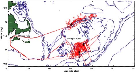
All of the remaining drifter experiments and all of the dye experiments were performed during the second leg, 14 May to 7 June 1999. Table 2.1 is a time line of the main events. A detailed event log is in Appendix 10.4. The location of the experiments is indicated in Figure 2.1.
The various components of the experiment are described in the following sections, with some preliminary results.
Table 2.1 The Main Events of the Cruise
Cruise 323:
7 -10 May South flank surface layer drifter experiment
7 - 9 May South flank zig-zag surveys (3)
Cruise 324:
15-19 May South flank surface layer dye/drifter experiment
20-22 May South flank surveys
23-28 May South flank pycnoline dye/drifter experiment
27 May South flank ROV-based plankton studies
29 May North flank survey
30-31 May North flank pycnocline preliminary drifter experiment
31 May North flank ROV-based plankton studies
1 - 6 June North flank pycnocline dye/drifter study
Figure 2.1 Ship track for EN323/EN324. The bold numbers along the tracks indicate the approximate locations of the four dye releases.
LEG 1
Initial Surveys: May 6-12
R/V Endeavor departed Woods Hole at 1915 EDT on 5 May 1999 for the south flank of Georges Bank. Tests were performed on the way with the Video Plankton Recorder (VPR) towed body to adjust the trim. A survey of the south flank began late on 6 May and continued through most of 7 May. (See Survey 00 in Section 10.6; Cruise tracks are shown in Section 10.6 and are organized and referred to herein as "surveys." A shorthand description of the survey is in Table 10.5.1.) This was a zig-zag survey extending between the 50-meter and 75-meter isobaths and from 10 km east of the Schlitz Tidally Mixed Front mooring line to 45 km west of it. Just to the west of the mooring line, five drogued and surface drifters were released on the morning of 7 May. The water column was found to be very weakly stratified below approximately 6 m depth, even south of the tidal mixing front, which was defined as the location of a strong off-bank temperature and salinity gradient in the surface water, and was near the 60-meter isobath.
A second survey, similar to the first, was performed between the mornings of 8 May and 9 May during the first drifter experiment (Survey 01, Sec. 10.6). Then tow tests were performed with the dye fluorometer and Wet-Labs AC-9 absorption/attenuation meter to adjust the trim of the towed body and then to measure the background fluorescence detected by the fluorometer. These measurements ended on the afternoon of 9 May, and were followed by a test of the dye injection system.
VPR survey 3, a somewhat abbreviated repeat of the previous surveys, was performed between 2100 EDT on 9 May and 1600 EDT on 10 May (Survey 03). Also on 10 May, the five drifters that had been deployed were all successfully recovered, with a CTD cast performed at each recovery location. (See Sec. 5 for a discussion of the findings from this and the other drifter deployments.) A fourth VPR survey, begun at 2300 EDT on 10 May, was to be a site survey for the first dye release. However, an encounter of the towed body with the bottom at 0100 EDT on 11 May precipitated a failure of the VPR winch. The towed body was recovered with the aid of a capstan at around 0430 EDT. An ADCP survey to the east of the Schlitz mooring was undertaken during the day on 11 May while work was done on the winch. At 1530 EDT it was decided that it was necessary to return to Woods Hole for winch repairs, and the ADCP survey was terminated. The ship arrived in Woods Hole at 0830 EDT on 12 May for a two-day break to repair the winch. This port break was substituted for one that had been scheduled for 25-27 May. The interruption of the cruise came at a reasonably good time, since the first drifter experiment had been completed and the first dye/drifter experiment had not been started.
Drifter Deployment #1 - May 7-11
In this first drifter study, our aim was to explore convergence onto the tidal mixing front from both the stratified and unstratified regions. Towards this end, we deployed drifters in the frontal region and on either side of the front. (See Table 5.1a for a summary of drifter deployment/recovery locations and times.) Deployment operations began on the morning of May 7 by steaming NNW and marking the passage of the front, as identified by the readouts of the ship's 1 m and 5 m thermistors. The first drifter, a surface follower, was set in vertically well mixed water ~8 km NNW of the front. We then steamed SSW and deployed four additional drifters. Two were set in stratified water near the tidal mixing front. One was a surface follower and the other was drogued at a mean depth of 19.4 m (see the Drifter Section, starting on page 17, for a description of the different types of drifters). The other two drifters, also a surface follower and 19.4-m drogued unit, were set in vertically stratified water 7 km further to the SSW. Unfortunately, the surface drifter set at the front, #8, only transmitted once after being released. This was a remarkable "come and get me call" which was sent more than 3 days after deployment (during recovery operations) and extended over a number of miles, further than the usual drifter transmission range to the R/V Endeavor. A preliminary discussion of the trajectories is in Section 5.
LEG 2
VPR Surveying - May 14-16
R/V Endeavor left Woods Hole again at 1600 EDT on 14 May 1999, and headed to the southern flank of Georges Bank by way of the southern route around Nantucket Shoals. The first data collected were from an ADCP line, which roughly followed the 80-meter isobath and started around 0230 EDT. The ship speed was at first too great to obtain good data, but was later reduced to around 9 knots to obtain 75% data return at a propeller speed of 160 rpm. Apparently, the propeller speed must be reduced to 140 rpm to obtain near 100% data return. During this line, the VPR was trimmed for 8 knots with a new mount for the Chelsea rhodamine fluorometer, the AC-9 having been removed from the sled. By the time we reached the southeast corner of our large-scale sampling track, trimming was complete, and we began to obtain VPR data on the line just east of the Schlitz mooring array. This line was interrupted by a visit from a party from the Edwin Link to exchange information and data with us.
The line was then continued to its northern end, where we paused to perform an inter-calibration of the CTD sensors on the dye injection sled and the VPR. It was found that the temperatures differed by 0.03 C, and the salinities also differed. Appendix 10.1 deals with CTD Sensor Calibration.
The survey north and west of the mooring array continued until the VPR winch began to shut down mysteriously and with increasing frequency. The problem was found to be arcing across the leads to a control solenoid and was fixed by 0500 EDT on 16 May. At this point, we shifted from the large-scale VPR survey to a smaller-scale survey around the prospective site for the tracer release, across the tidal mixing front and west of the mooring array. During this survey we discovered that the stratification just east of the array was much better developed than to the west. To the east of the moorings, there was a mixed layer 5 to 10 meters deep overlying a pycnocline of similar thickness; while to the west the entire mixed layer was barely 5 meters thick. However, finding abundant Calanus in the west, and wishing to avoid running into the moorings during sampling, we opted to release the dye in the western region of less well developed stratification.
Southern Flank Surface Dye Experiment, and Drifter Deployment #2 - May 16-19
Prior to the surface dye release, a surface drifter was set near the tidal mixing front, the location of which was identified from the readouts of the Endeavor's 1-m and 5-m thermistors. The dye injection commenced roughly 1.5 hr after the deployment of this drifter. The dye was released from 1322 to 1431 EDT on 16 May 1999 into the shallow warm layer and approximately 6 km SSW of the tidal mixing front. 120 kg of Rhodamine WT were released at 3 meters depth with the ship heading 060 to 065 degrees at 0.2 to 0.3 m/s directly into a light wind. The resulting ship track was 1580 m long heading 030 degrees at 0.38 m/s relative to the motion measured by the shipboard ADCP at 11 m depth (Survey 10). This relative motion suggests the effect of wind on the ship, or the presence of a shallow Ekman layer, or both. The track in coordinates fixed to the earth was completely different, with a course of 101 degrees and length 3300 m, due to the tide. The tidal flow, which was at the height of the spring-neap cycle, was just turning off-bank.
The dye was released into a stratified layer about 5 meters thick, over which the buoyancy frequency increased with depth. Below the base of this layer, the buoyancy frequency was very low all the way to the bottom of the cast (The VPR tow-yos end 10 to 15 m above the bottom). The dye was released along side the starboard waist of Endeavor, the 3-meter depth being shallower than the draft of the vessel. The bottom of the propeller blade on the Endeavor is at 5.7-meter depth. Some of the dye passed directly though the propeller wash, and all of the dye was no doubt affected by the wake of the ship.
During the dye injection, three surface drifters were deployed into the dye patch. Each was released during a dye barrel switchover (when the injection plumbing was switched from an emptied to a full dye barrel). Specifically, the releases occurred after injection of 1, 2 and 3 (out of four) barrels of dye. (See Table 5.1b for drifter release locations and times.)
The density of the dye mixture at 10°C was 1022 kg/m3, while the density of the water at the CTD during release ranged from 1024.7 to 1025.2 kg/m3. Hence, the dye mixture was light relative to the water, and might be expected to rise to the surface. However, the density anomaly of the dye would have been reduced by a factor of more than 100 by dilution into the wake of the injection sled within a minute or so. The variance of the initial density of the tagged water would have been due mostly to the variance of the density passing the injection sled and the turbulence due to the wake of the ship and the propeller.
The initial dye plume was readily observed from the deck of the ship, to the entertainment of all hands. Aft of the release system, along the starboard side, the dye took on a brain-like texture, lying some 1 to 3 meters beneath the surface, with sharp boundaries between the dyed and undyed water. There were also some more diffuse clouds of dye. Dye that passed through the propeller was mixed to the surface, with brain-like features obliterated. Observed from the upper decks, the overall dye streak lay in a eddying line more or less straight back from the ship (Fig. 3.1). There was an appearance of the deeper dye lying to the starboard side, and the shallower dye lying straight back, or slightly to port, again suggesting a shallow Ekman flow.
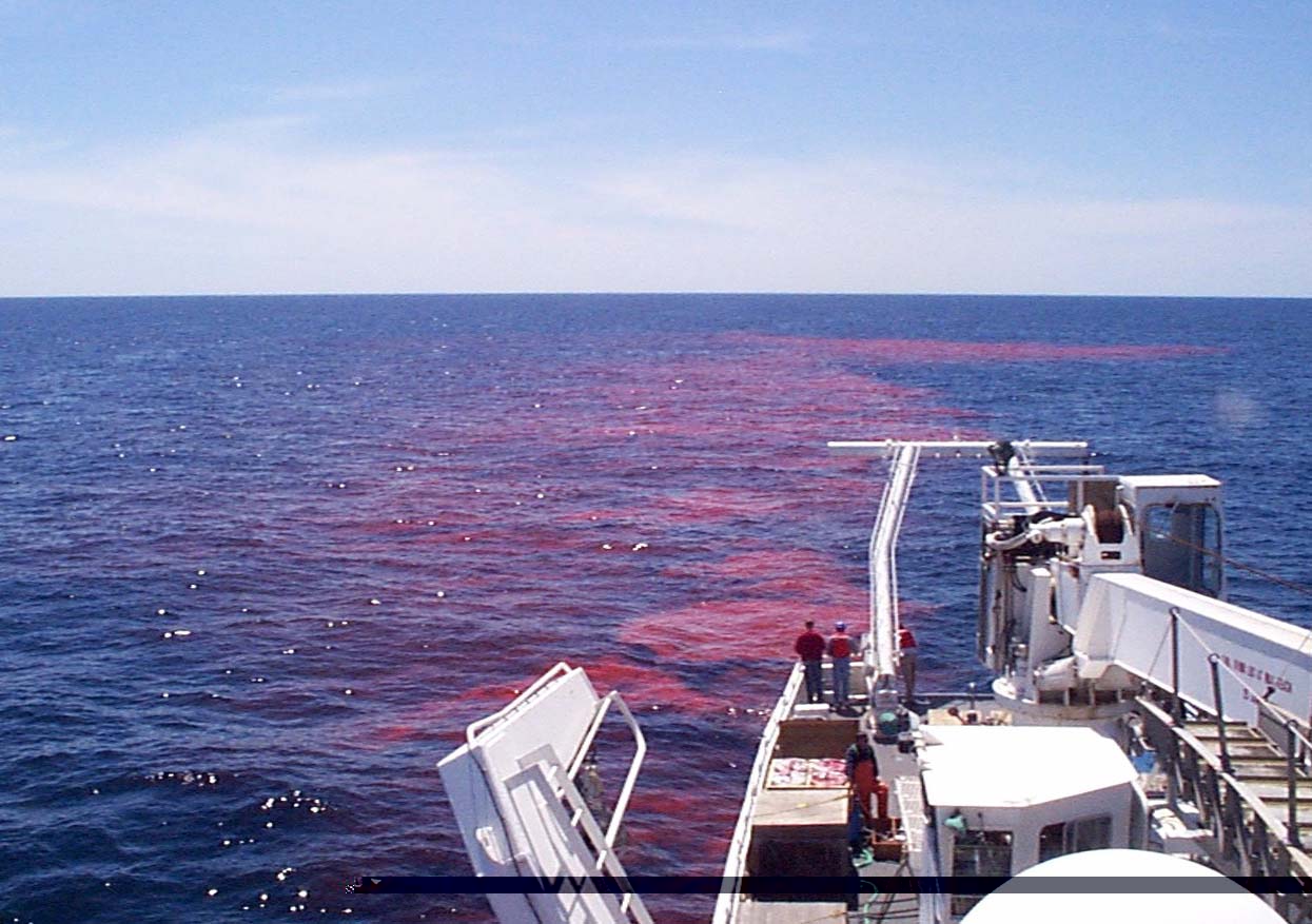
Figure 3.1 Surface dye release as observed from the bridge of the R/V Endeavor
Once the release was completed, the release system was recovered and the VPR was deployed for initial sampling. The ship circled back to begin sampling at the most recently released dye and to work back toward the start of the plume. Five crossings of the dye patch were made, of various lengths through the patch, between 1543 and 1742 EDT; i.e., 1 to 4 hours after release (Survey 11). The dye was found 700 m north of its position predicted from the 11-meter ADCP record at the eastern end and 2800 m north at the western end, evidence of a northward surface velocity of nearly 20 cm/s relative to 11 m.
The Endeavor steamed north to locate the front, which was found to be just 3 km north of the dye patch. On the way back to the patch, a surface drifter was deployed, approximately half way between the front and the patch. Another drifter was deployed ~2 km to the south of the patch (Table 5.1b). With night descending, a second survey of the patch was started (Survey 13). During this survey, which continued into the afternoon of 17 May, the position of the front was checked approximately every 6 hours. The survey data revealed that the shallow, western part of the patch made its way into the mixed zone. The surface drifters deployed south of the front were also carried into the vertically mixed zone. Presumably both the dye and drifters were carried by the Ekman current generated by the easterly wind. The part of the patch found south of the front was divided into a surface patch and a 5-10 m deep patch further from the front. Later in the survey, concentrations above background appeared in the deep water to the southwest, increasing as the VPR approached its maximum depth of 15 or 20 meters above the bottom. The source of this signal must be explored.
After a brief trial of the ROV in seas judged to be too rough, the third and final survey of the patch was conducted from 17 May to 19 May. This was planned as a radiator pattern, covering a broader region than was believed occupied by the patch. Fifteen-km lines were occupied, running from the front at a heading of 160 degrees, with return lines up to and beyond the front at the reciprocal heading of 340 degrees (Survey 14). Just before starting this survey, elevated dye concentrations were found in a small area in the surface warm layer near the front. The survey encountered relatively low dye concentrations over a broad area, both on the mixed side of the front and on the stratified side below the warm surface layer. These concentrations were 0.005 to 0.03 ppb, near the minimum detectable level of 0.01 ppb. It was only by their spatial pattern that we surmised that they were not due to background interference. After the survey, we returned to the area where elevated concentrations had been measured prior to the survey. They were no longer to be found. Presumably by this time, all the dye had either been advected into the well mixed zone or had remained in the stratified zone and mixed downward into the unstratified water beneath the warm surface layer. It seemed that a sizeable fraction of the total dye had left the surface later in one of these ways, the shallower dye to the mixed zone, the deeper dye to the deep layer.
At the end of this final survey, we occupied a line back and forth to the 1000-meter isobath (on the upper slope), gathering ADCP and plankton data. The hydrographic structure was complex, due to the presence of Gulf Stream and/or slope water intrusions.
During the afternoon of 19 May, upon our return from the slope, we recovered all six of the drifters. The operation was completed over a period of 5 hours. CTD measurements indicated that all drifters were retrieved in the vertically mixed zone.
Afterwards, with the weather barely allowing it, we deployed the ROV for some tantalizing glimpses of the plankton at low flow past the cameras. However, the swell was high and the wind-induced drift of the ship was considerable, making it difficult to maintain slack in the ROV tether.
VPR Surveying - May 20-23
Early on 20 May we began a repeat of the large-scale VPR survey, going from east to west (Survey 15). It was noted that the fluorometer was becoming noisy on the upcasts, presumably due to mechanical vibrations. With the ship moving at 8 knots, sled speeds on the upcasts can reach 10 knots. It was also noted that there was relatively high fluorometer background toward the south edge of the survey, associated with patches of high chlorophyll. On 21 May, the large-scale survey blended into a local survey to the west to find a promising site for the second dye experiment (Survey 16). The hydrography appeared promising, with a well developed mixed layer and pycnocline west of the Schlitz mooring line. Committed to release the next day, because of the desire to coordinate releases with Oceanus, we continued surveying to the west, where a rich patch of Calanus was found and mapped well. Tows were performed at constant density to measure the spatial variability within the patch.
Returning to the area just west of the Schlitz mooring line on the morning of 22 May (to join Edwin Link and Oceanus in a three-ship operation), we had difficulty finding a good site for the second dye release (Survey 09). In places the Calanus were abundant, but the pycnocline was 1 to 2 meters thick, an impossible target for the dye release. In other places, the pycnocline was thicker but the Calanus abundance was very low. With the day drawing on, we decided to postpone the release for a day, to allow for a thorough survey of the possible release region. We surveyed all night, at first to the east almost up to the Schlitz moorings where very low Calanus abundance was found. We passed over the dye patch from the Oceanus and found that we could see a signal from their fluorescein in our rhodamine fluorometer. Not wishing to interfere with the Oceanus' experiment, we decided to moved well to the west of their dye patch, on the supposition that our pycnocline patch would drift west faster than their bottom patch. Our survey in the west (Survey 010) found the Calanus abundant and the thickness of the pycnocline generally greater, and so we selected a site at which to perform our second release.
Hydrographic sections across the south flank of the bank revealed a thin warm surface layer well onto the bank crest, and a thicker warm surface layer ending at the 60-meter isobath. Since heavy winds were anticipated for the 24 hours after the dye release, we expected the thin warm layer would be eroded completely and that the "true" front would move back to the 60-meter isobath. Accordingly, we chose a spot for the second tracer release that was approximately 9 km south of the edge of the thick warm layer, and 15 km south of the edge of the thin warm layer. There were abundant Calanus at this spot. It turned out that the wind did not move the edge of the warm layer back toward the release point, perhaps because it was such a warm wind. If anything, the wind thickened the warm layer that had been thin. Hence, the release point ended up being 15 km south of the surface expression of the front.
1st Southern Flank Pycnocline Dye Release,and Drifter Deployment #3 - May 23-29
The target potential density for the second dye release was 25.295 (VPR sensors), which had been the density characterizing the edge of the front below the thin warm layer. The release was performed in a manner similar to that for the first release, with light wind off the starboard bow and speed through the water of 0.2 to 0.4 m/s (Survey 20). With the calm weather, we were able to hold the CTD on the target isopycnal with a rms error of 0.016 kg/m3. Given the mean vertical density gradient of -0.058 kg/m4 (N = 13 cph), this error corresponds to a rms depth error of less than 0.25 m. It was important to be accurate because the thickness of the entire pycnocline was no more than 5 meters.
There were two interruptions of the release. After 10 minutes of pumping, a fuse blew in the control system, causing a 5 minute cessation of the release. Later, the pumps lost suction for two minutes. Finally, between the third and final drum of dye, the line became clogged somewhere. Not wanting a large gap in the injection streak, and feeling that we had injected enough dye, we terminated the release, saving the last drum for later. The total amount of Rhodamine-WT injected was approximately 65 kg.
Roughly 2.5 hours prior to the dye release, a surface drifter was set out in slightly stratified water (8.8 °C at 1m and 7.4 °C at 5m) near the front. The dye was injected roughly 16 km to the SE of this drifter. Four drifters were released during dye injection. Drifters drogued at 19.4 m were set out after the release of 1, 2 and 3 barrels of dye, and a surface drifter was set out after the third (and final) barrel. Unfortunately, one of the drogued drifters, #10, ceased transmitting to ARGOS after a little more than a day on the job.
The VPR was deployed very quickly after the end of the dye release, and the ship began to return to the most recent end of the streak. The first dye was found approximately one hour after the end of the release. A series of lines was occupied across the streak, using headings of 160 and 340, and sharp turns between at a ship speed of 2.5 knots (Survey 21). Within a few hours the survey was complete, and the patch appeared to be delimited. Extra sampling effort was made to make sure that the dye released in the first 10 minutes, before the fuse blew, was not separated from the main patch and lying in an unsampled patch elsewhere. About 20% of the dye was released in this subpatch, and the ship had moved rather far during the 5-minute gap.
The survey found the dye centered at the target isopycnal surface. However, the vertical spread seemed large. There were lobes in the deep part of the pycnocline, and it was even apparent that some dye had mixed below and above the pycnocline. It was also noticed that there may be a lag in the fluorometer, at least relative to the pressure on the VPR sled, since the dye seemed to be found deeper on the down casts than on adjacent upcasts.
Upon completion of the first survey, a VPR line was done to the tidally mixed front (Survey 22). This was followed by a VPR line back through the dye patch and further to the south. During this VPR survey, a drifter was released at the patch. Its drogue was set at a mean depth of 39.4 m so that it would always reside in the subpycnocline water beneath the patch. A final drifter, drogued at the mean pycnocline depth of 19.4 m, was set out in the stratified water roughly 3 km south of the dye patch.
This operation was followed by a VPR survey carried out on 10 x 10-km radiator pattern roughly centered on the dye (Survey 23). This was done to obtain the Calanus and hydrographic structure on a larger scale than was obtained during the previous dye surveys. Also during this period, the ROV was deployed and obtained excellent views of the Calanus in their natural habitat.
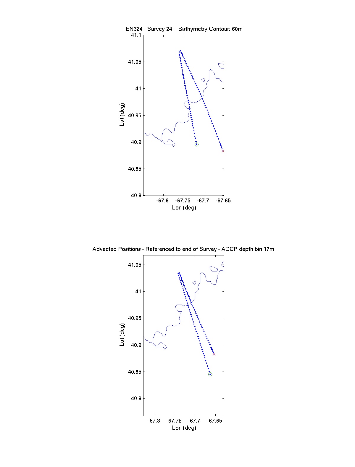
After this survey, on the night of 24 May, another VPR survey line was run to the front, which was encountered 16 km to the north of the patch (Survey 24). The warm layer observed near the front on the previous night had been mixed downward by a day of 25 to 30 knot winds, but the density at the front remained unchanged.
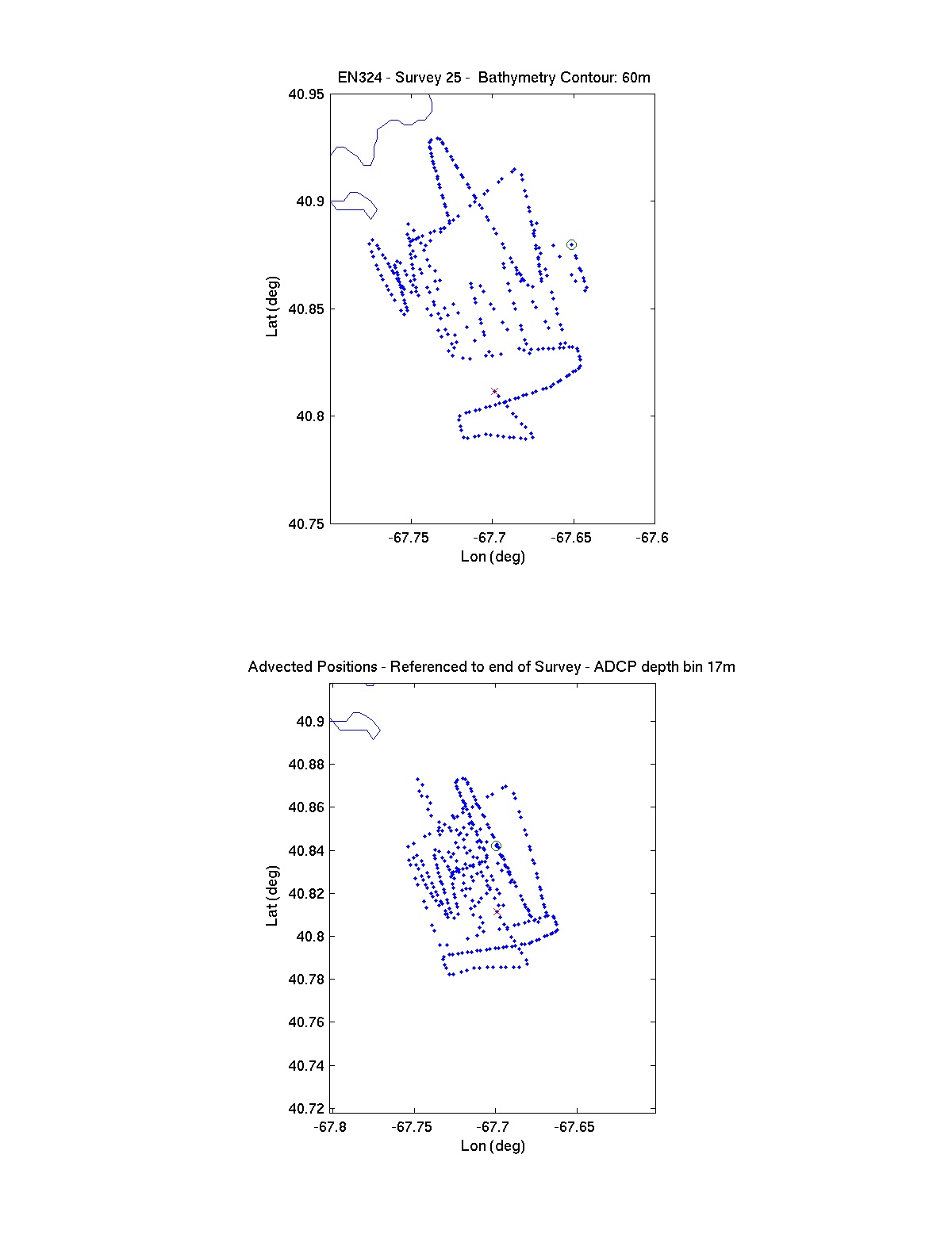
This excursion to the front was followed immediately by the second systematic survey of the dye patch (Survey 25). The main part of the patch, in the pycnocline, was found to extend 5 km in the along-isobath direction and 3 km in the cross-isobath direction. There appeared to be elevated concentrations in the deep water north of the patch and at the base of the mixed layer south of the patch, suggesting shear. How much of this was due to tidal motions and how much was subtidal remains to be determined. Also, it was sometimes questionable how much of the shallow dye signal was due to interference. The signal did seem strongest south of the center of the patch, decaying to the east and west with the patch, but the southern limit of the signal was not found. Later in the cruise, similar large false dye signals were found at the base of the pycnocline.
On the excursion to the front after this survey, we found the thin warm surface layer had been restored by the day's heating and moderate winds. The distance to the front was still around 16 km, but the density at the front had decreased to 25.175 (VPR). The density beneath the patch, on the other hand, remained near 25.51, as in the initial survey. Hence, it appeared that the patch had not moved relative to the front or to the deep density field.
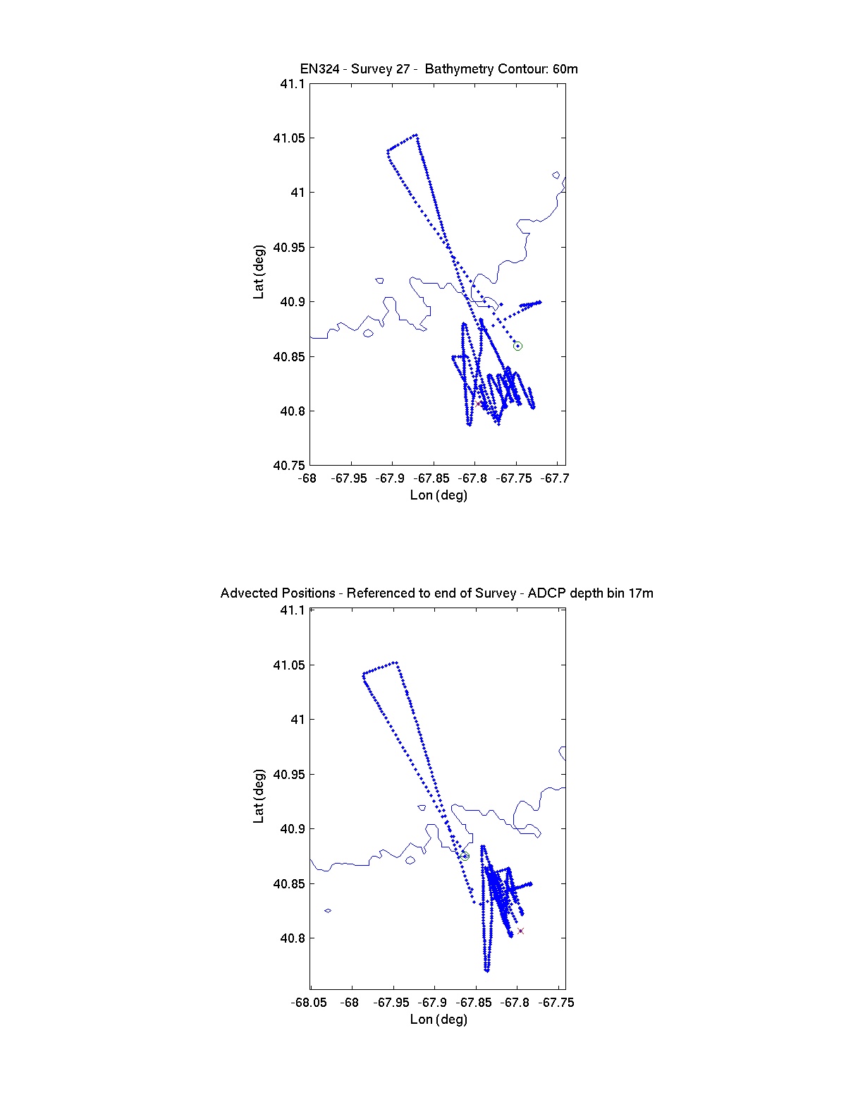
Upon returning from the front, we undertook a 25-hour study (from 1900 on 25 May to around 2000 on 26 May) of layering and diel migrations of plantonic communities (Survey 27). This study yielded novel information on how the species are layered relative to one another and how they change position during the diurnal cycle.
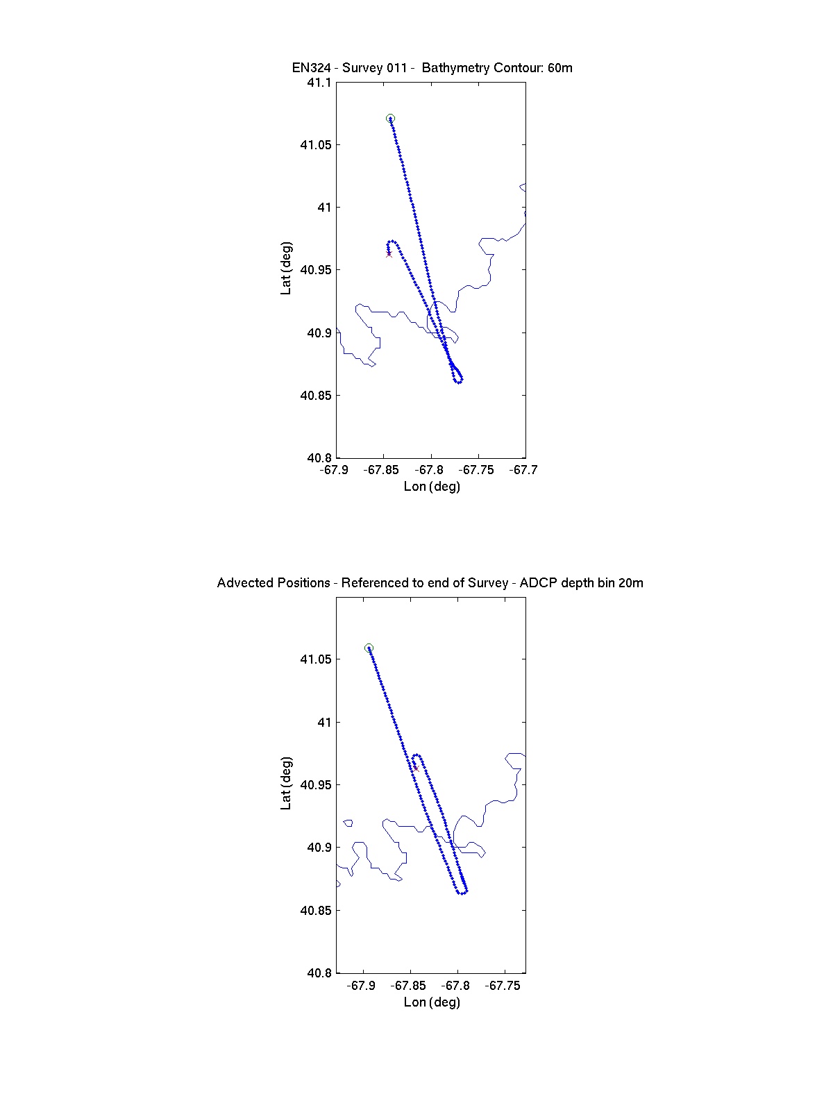
After this 25-hour study, another section was run from the patch to the front (Survey 28). This was followed by recovery of a drogue well into the mixed zone. We then returned south to the front, towing the VPR at a constant depth to accurately delineate the horizontal front of chlorophyll and planktonic communities (Survey 011). This operation was repeated going north through the front again. In search of a site for a second pycnocline dye release, we then ran two sections across the front while tow-yoing the VPR (Survey 012).
2nd Southern Flank Pycnocline Dye Release - May 27-29
We decided to try a second dye release in the pycnocline closer to the front, with the dye left over from the 1st pycnocline release. The dye release site chosen was approximately 6 km south of the edge of the front. The density sq at the edge of the front was 25.230 (VPR), with no warm layer whatsoever on top. At the site chosen, this isopycnal surface lay between 10 and 20 meters depth, with a little stratification below and above. Because of the offset between the VPR and Sea-Bird CTD sensors, the target was at first adjusted to 25.250 prior to release. However, after measurement of the density profile by the deployment CTD, we decided that there was too little stratification below the 25.250 surface, and reverted to a target of 25.230 (Sea-Bird). The injection went fairly smoothly. It was, however, difficult to maintain the sled at the target density, due to a sharp vertical density gradient at the target.
Approximately 23 kg of dye were injected, i.e., one of our barrels. The streak was 500 meters long and lay in the along-isobath direction, i.e., at a heading of 250 degrees relative to the moving water according to the ADCP record (Survey 30).
Immediately after recovery of the injection system, the VPR was deployed and the ship was brought back to the streak, crossing it from the north. We found the first dye peak 41 minutes after the end of the injection. Three crossings of the dye streak were made, with 6 to 10 profiles obtained on each crossing (Survey 31). The dye appeared to be spread throughout the pycnocline. How much of this was due to lag in the sampling system and how much to imperfections in control and the wake of the injection system remains to be evaluated. Some dye peaks were within 3 m of the surface, others were at depths greater than 20 m.
At the end of the third crossing, a drifter, drogued at 14.4 meters, was deployed to mark the patch. We then steamed east to recover one of the drifters that had been released within the second dye patch. Afterwards, we attempted to locate the second dye patch for ROV observations of the plankton. Upon our return to the area of the second patch, we found the foot of the shelf-slope front, and rather weak dye signals in the pycnocline which could have been background. Turning north, we saw this small signal grow to as much as 0.5 ppb of dye, which was presumably the real thing, and then decrease again. Without further searching, the ROV was deployed in a rich patch of biota. The wind was light and excellent observations of Calanus were obtained by the ROV video system.
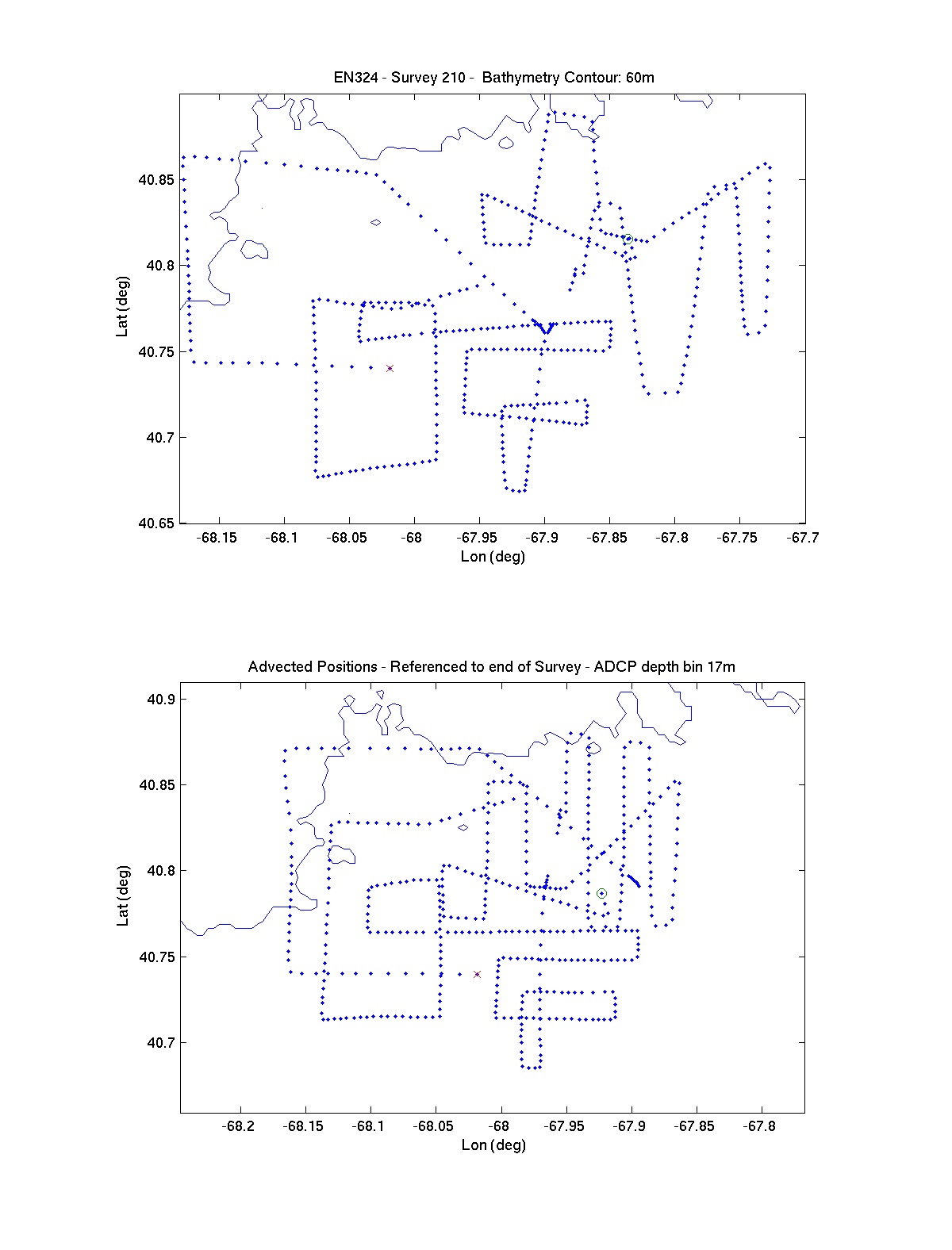
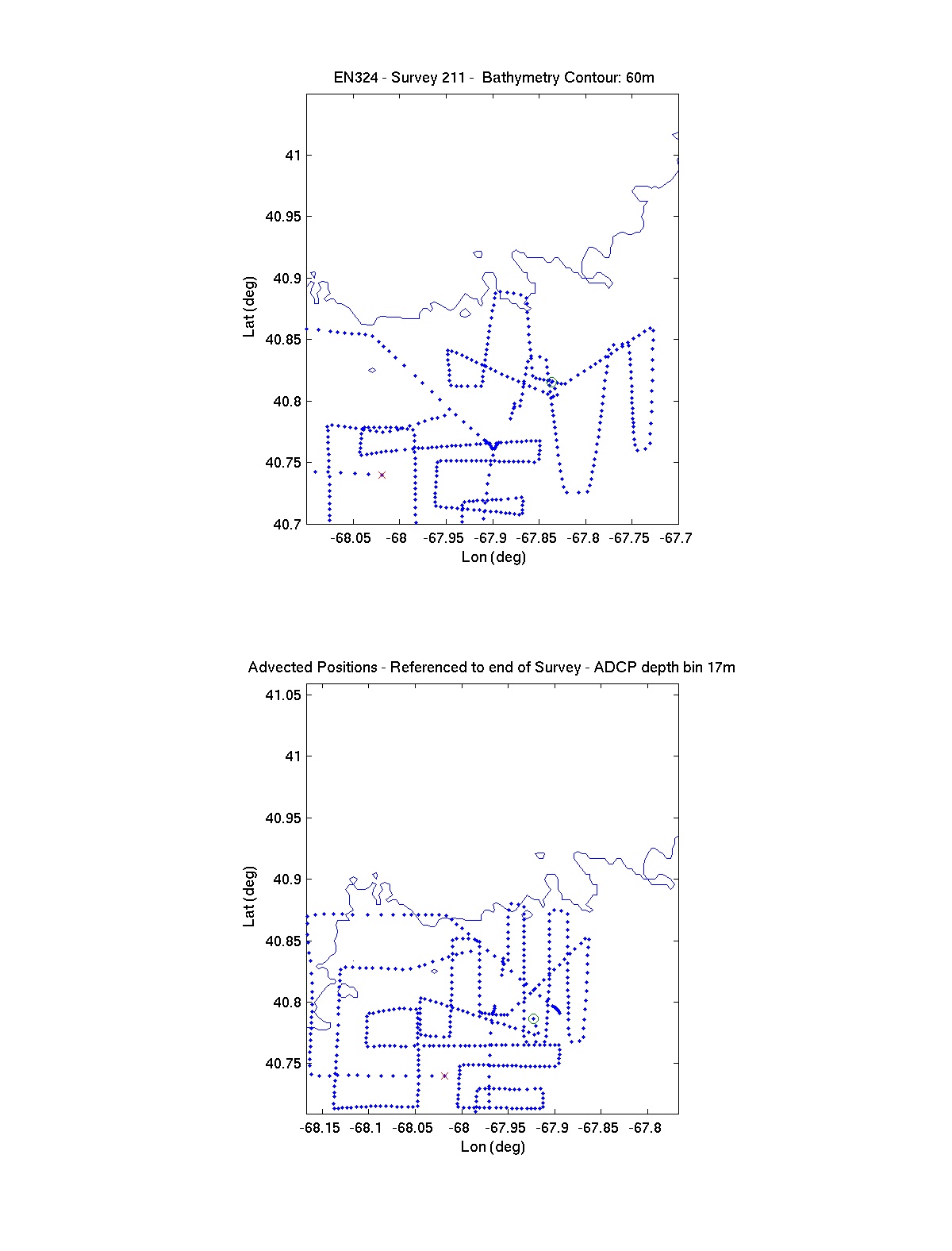
The third systematic survey of the dye patch ensued, from the night of 27 May to the night of 28 May, with an interruption to recover three drifters. Rhodamine signals were low throughout this survey and were difficult to distinguish from background. Nevertheless, a patch of elevated signal was identified and nearly delimited. This patch included location of the dye patch as projected from the observations earlier in the week by the ADCP record. It extended north and then west from there, and then possibly north again. This northern lobe toward the west end of the patch may be difficult to distinguish from background, although T/S properties may help (Survey 210; Figure 4.1).
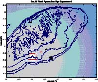
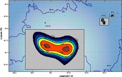
Figure 4.1 Pycnocline Dye Experiment on the South Flank.
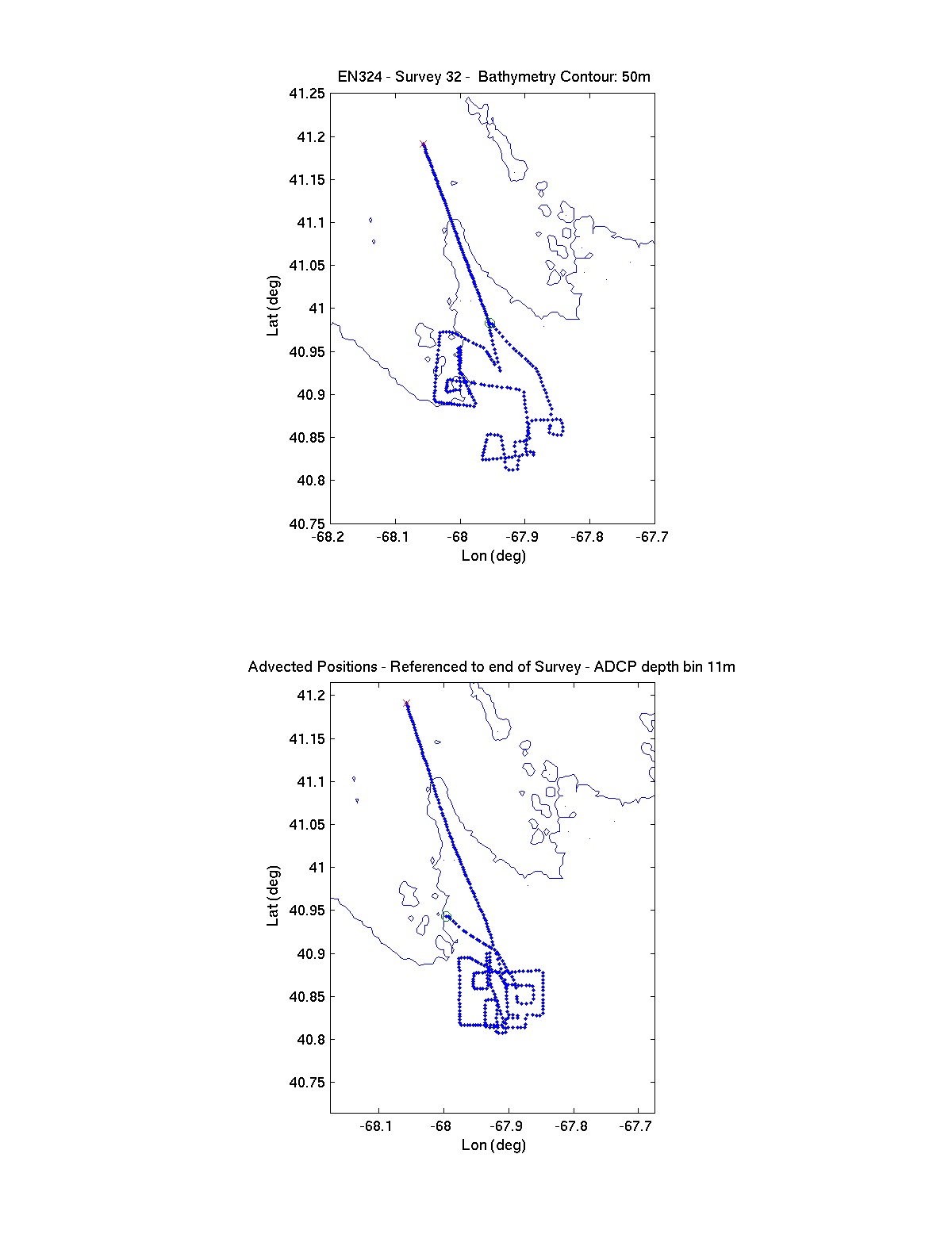
A final section from the main dye patch to the front was occupied at the end of this survey. Then, early on 29 May, we proceeded to the position of the drifter deployed two days earlier to mark the small dye patch near the front. A search around the drifter found very weak dye signals (Survey 32). The only signal that could be distinguished from background was within 5 meters of the surface, in a band north of the drifter. There was a hint of dye spread from pycnocline into the deep waters south of the drifter. Apparently vigorous mixing had weakened the signal to less than 0.06 ppb, not a surprising result given that the amount released was just 23 kg and the time elapsed since release was 2 days.
After this survey of the small patch, we recovered the drifter deployed in the patch, and then ran a section toward the crest of the bank. On this section, we found a light surface layer of warm water occupying the upper few meters well onto the crest. Although the moon was nearly full, the wind had been light and the skies clear for solar heating. This observation reminds us that the well mixed zone is not always well mixed, even during spring tides. There can be a thin cap of light water, which unfortunately could confound the interpretation of measurements made from the air or from space.
VPR Surveying of the Northern Flank, and Drifter Deployment #4 - May 29-31
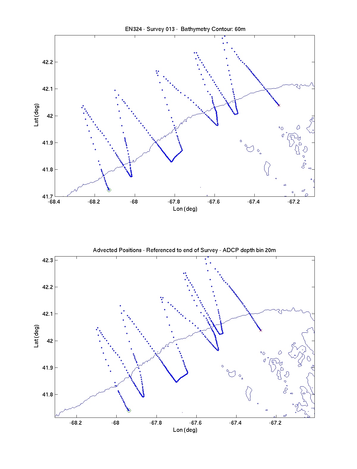
This section onto the crest marked the end of our work on the south flank and our departure to the north flank. Late on 29 May we began a large scale survey of the north flank, with 36-km lines running approximately cross-bank in a zig-zag pattern from 68 W to just west of the Hague Line. This pattern was completed late on 30 May (Survey 013).
Early on the morning of 30 May, we deployed three drifters over the slope off the northern flank (Table 5.1d). The first, drogued at 19.4-m, was set out in stratified water roughly 7 km from the 60-m isobath. The other two, a surface and a 19.4-m drogued drifter, were set roughly 2.7 km further north (9.7 km from the 60-m isobath).
The early morning of 31 May (0400-1200 EDT) was devoted to ROV operations, for which sea conditions were excellent. The ROV was deployed at three stations. At the most off-bank station, relatively low concentrations of organisms were found. At the middle site, over the slope, a high abundance of C. socialis was encountered. Numerous colonies of C. socialis were also seen at the final site, within the mixed zone on the bank crest.
In the afternoon and early evening of 31 May, we recovered the three drifters. The two drogued drifters followed very nearly the same trajectory, moving in the along-isobath direction at roughly 25 km/day and across-isobaths (toward the bank) at about 2 km/day. After the final drifter recovery, we began a high resolution VPR survey near 68°W, within the area of the prospective release site (Survey 015).
Northern Flank Dye Release and Drifter Deployment #5 - June 1-6
During the late morning of 1 June, we deployed five drifters along a line extending offshore of the northern flank and through the planned dye release site. Drifters drogued at 19.4 m were out over the 100, 186, 204 and 227-m isobaths, and a surface drifter was released at the 186-m isobath. The VPR was tow-yo'd at 4 knots between drifter deployments.
After the final drifter deployment, we steamed back toward the bank and commenced the dye release at a site over the 170-m isobath. Four barrels of dye, approximately 90 kg, were released between 1353 and 1447 EDT (near low tide) without incident, although the ship's track changed direction twice during release to avoid fishing traffic (Survey 40). This meandering made for a short initial patch. The target isopycnal was at sq=25.02 (Sea-Bird calibration) and about 20-m depth. At about the mid-time of the dye release (after two barrels had been emptied), two drifters were deployed. One was drogued at 19.4 m and the other was a surface drifter. Unfortunately, the drogued drifter ceased transmitting immediately after deployment. Later inspection of the drifter indicated that its main power connector had separated upon impact with the water.
Sampling of the dye patch with the VPR commenced immediately after the release(Survey 41). The dye appeared to be well confined in density, and centered at the target surface. During the initial survey, the malfunctioning drogued drifter was recovered, repaired, and re-released in the tracer patch.
Two other drifter incidents occurred during the dye surveying. On the morning of 3 June, the Endeavor received a radio call from the captain of the F/V Panther. He informed us that a fellow captain had picked up our drifter # 22. It lacked the drogue, which had apparently been cut free. After establishing radio contact with this second captain (the name of his ship was never recorded), we instructed him to redeploy the drifter, which then became a surface follower. He reported the redeployment site at 41°58.95' N and 67°58.54' W. Roughly two hours later, the captain of the Panther again contacted the Endeavor. Remarkably, he had dragged up the severed drogue of drifter #22. Upon our instructions, he returned the drogue to the deep but saved its thermistor, which he eventually mailed to J. Churchill. For these efforts, he later received our thanks in the form of a WHOI insulated jacket. The second drifter incident occurred on 4 June. During the early morning, the captain of the F/V Gulf Traveler reported, via radio, that one of our drifters had become entangled in a high flyer. He reported freeing it at 0815 EDT at a location of 42°07' N and 67°30' W. The drifter number was never recorded. However, based on inspection of the drifter tracks, it was probably drifter #6.
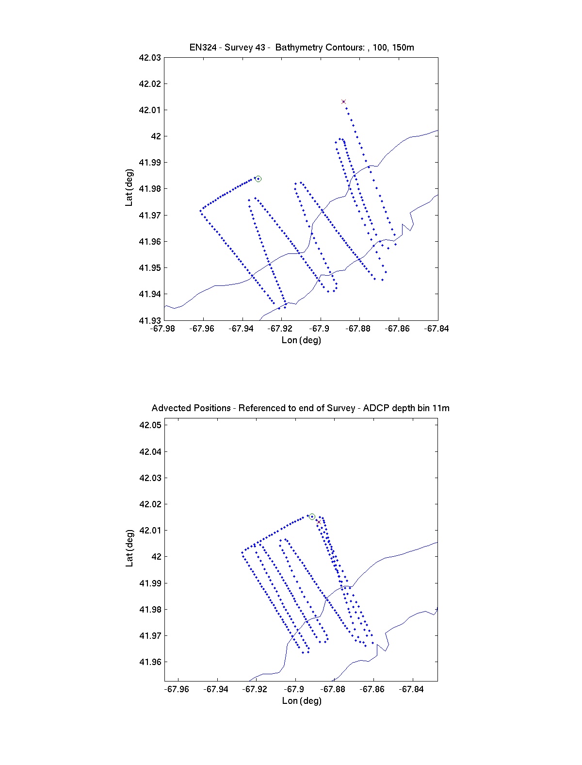
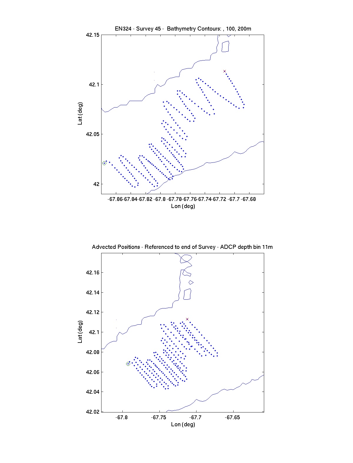
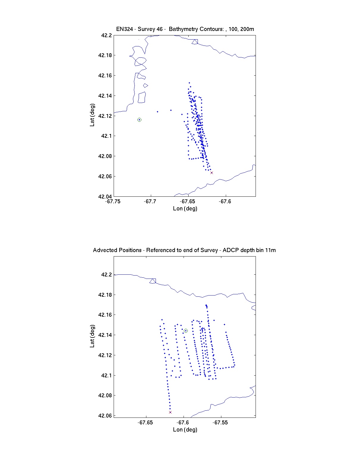
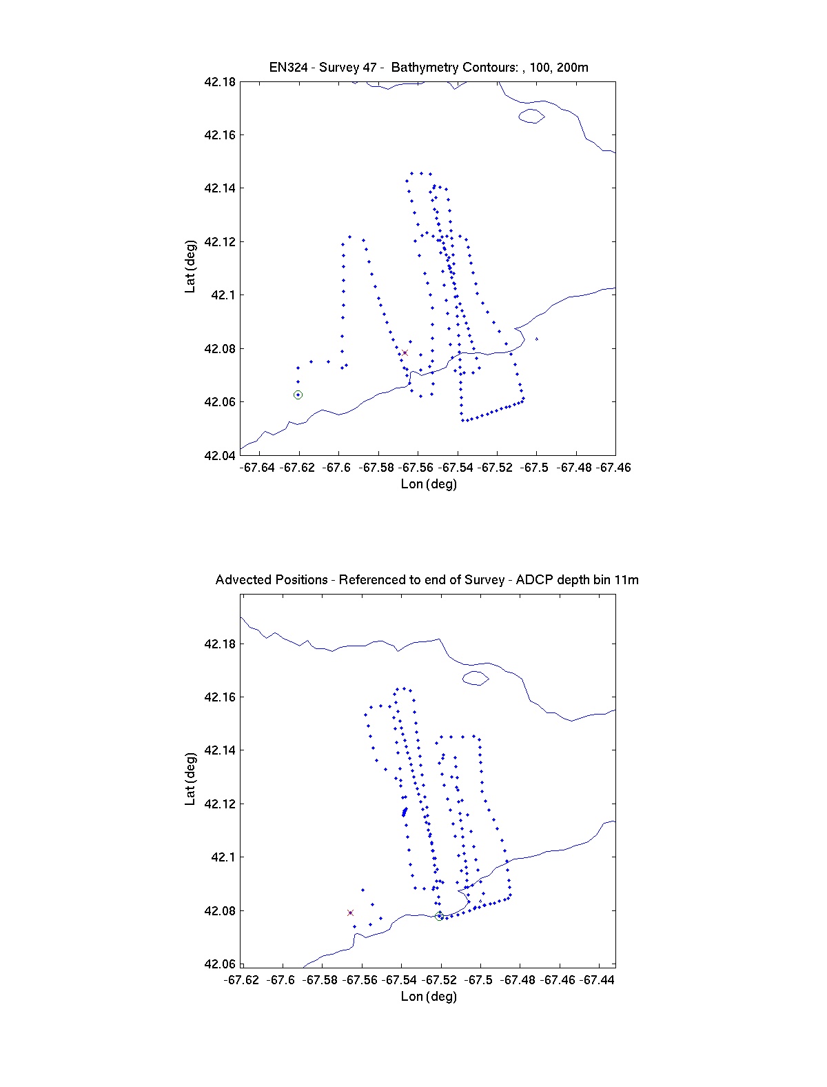
The patch was sampled more or less continuously until 6 June as it was advected along the North Flank at a speed of 20 to 25 cm/s (Surveys 42 to 49). The flow was predominantly along isobaths. The detided cross-isobath flow was highly variable in sign, and was ten times smaller in magnitude than the sub-tidal along-isobath flow.
Lying just below the dye patch was a thick patch of Chaetoceros socialis colonies, centered near the sq=25.3 isopycnal surface. This patch gave a large chlorophyll signal with no discernible dye background signal. Calanus abundance was low initially, but increased later in the experiment. Also later in the experiment it was found that where C. socialis dwindled to the north off bank, a source of chlorophyll from smaller organisms was detected. There was a slight background fluorescence signal associated with this community, but it promises not to interfere with the mapping of the dye, being too small and too far off bank.
While we were sampling the dye patch on 5 June, Bob Houghton on R/V Oceanus with some surplus time, kindly joined us. He surveyed the region between the 40-m and 200-m isobaths in the vicinity of our patch, hence probing the tidal mixing front and the currents across the North Flank. His survey, done between 0800 and midnight EDT, started near 66° 50'W, to the east of the patch, and proceeded west of the patch to near 67° 30'W.
Our sampling proceeded nearly continuously until around 1500 EDT on 5 June, when Endeavor was forced to stop for attention to carbon buildup in the turbine, caused by towing for many days at speeds mostly less than 6 knots. The engine had to be shut down for repairs. Fortunately, the seas were calm and the wind was light. We were back to normal operations by 1900 EDT.
The dye survey was continued into the early morning of 6 June, with the last clear signal, at the west end of the patch found just after 0000 EDT. After a few hours more of checking to the west, we commenced recovering the drifters that had been released with the dye. Four drifters were retrieved, and three were left behind as we steamed for Woods Hole.
James R. Ledwell, Terence G. Donoghue, and Cynthia J. Sellers
Injection
The fluorescent tracer used in these studies was Rhodamine WT, a dye designed specifically for water tracing. Injection of the dye after a suitable study area was chosen was accomplished with a unique containment, pumping and in-situ injection system. The containment system consisted of four 55-gallon drums within a water-tight plywood box. Rhodamine WT from the supplier, Crompton and Knowles, was delivered as a 20% Intracid solution. This solution was diluted and mixed ashore with isopropyl alcohol to adjust the density of the solution to within approximately 0.002 g/ml of the anticipated target surface, thermal expansion having been taken into account. The dual channel pumping system pumped dye from the barrels through garden hose tie wrapped to the hydrowire out a diffuser pipe attached to a small towed CTD package. Injection was maintained close to a target isopycnal surface by the winch operator, who had a video display to guide her. The pumps automatically shut down if the density at the CTD accompanying the injector strayed outside a preset window. Injection was continuous, barring malfunction, until the desired amount of dye is injected.
Sampling
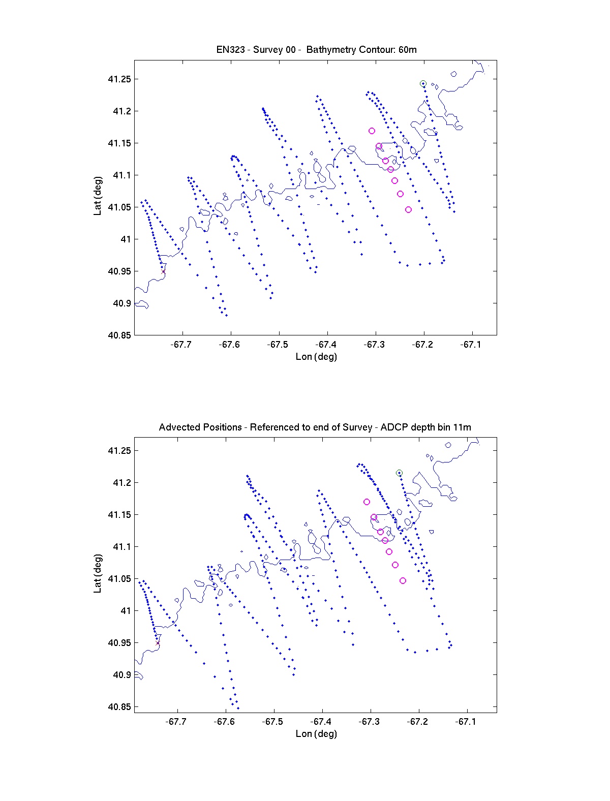
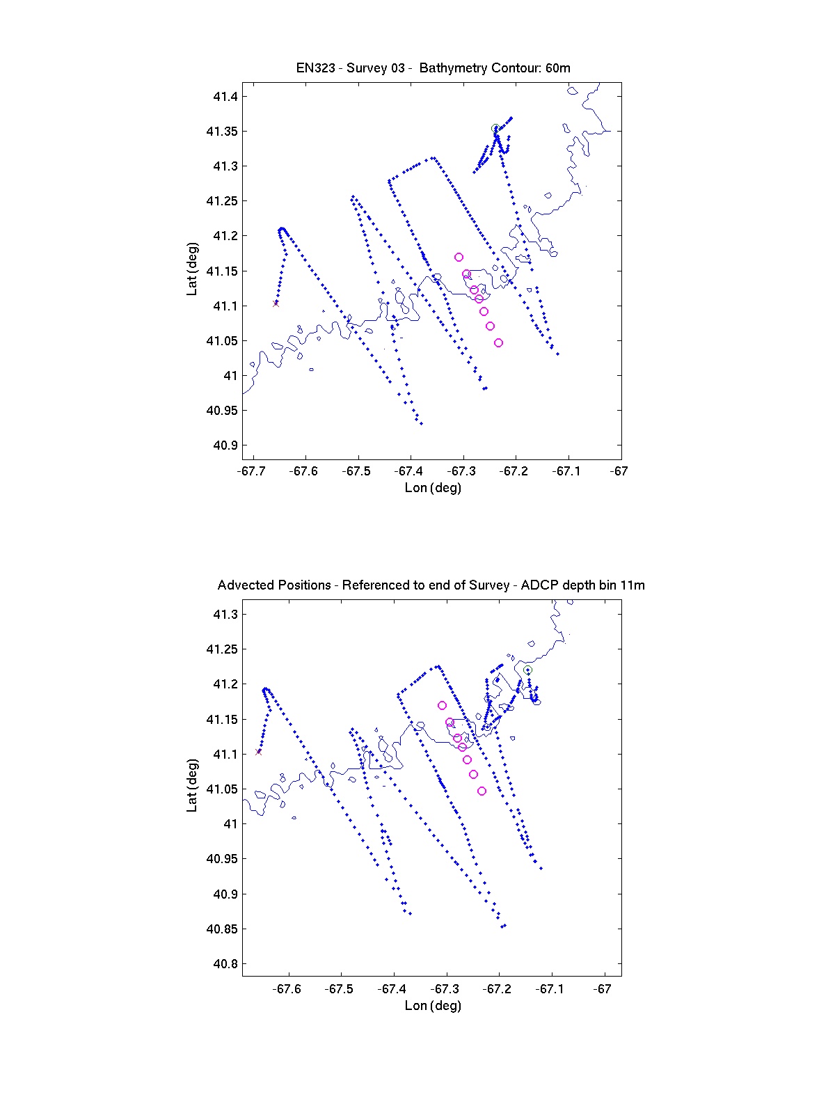
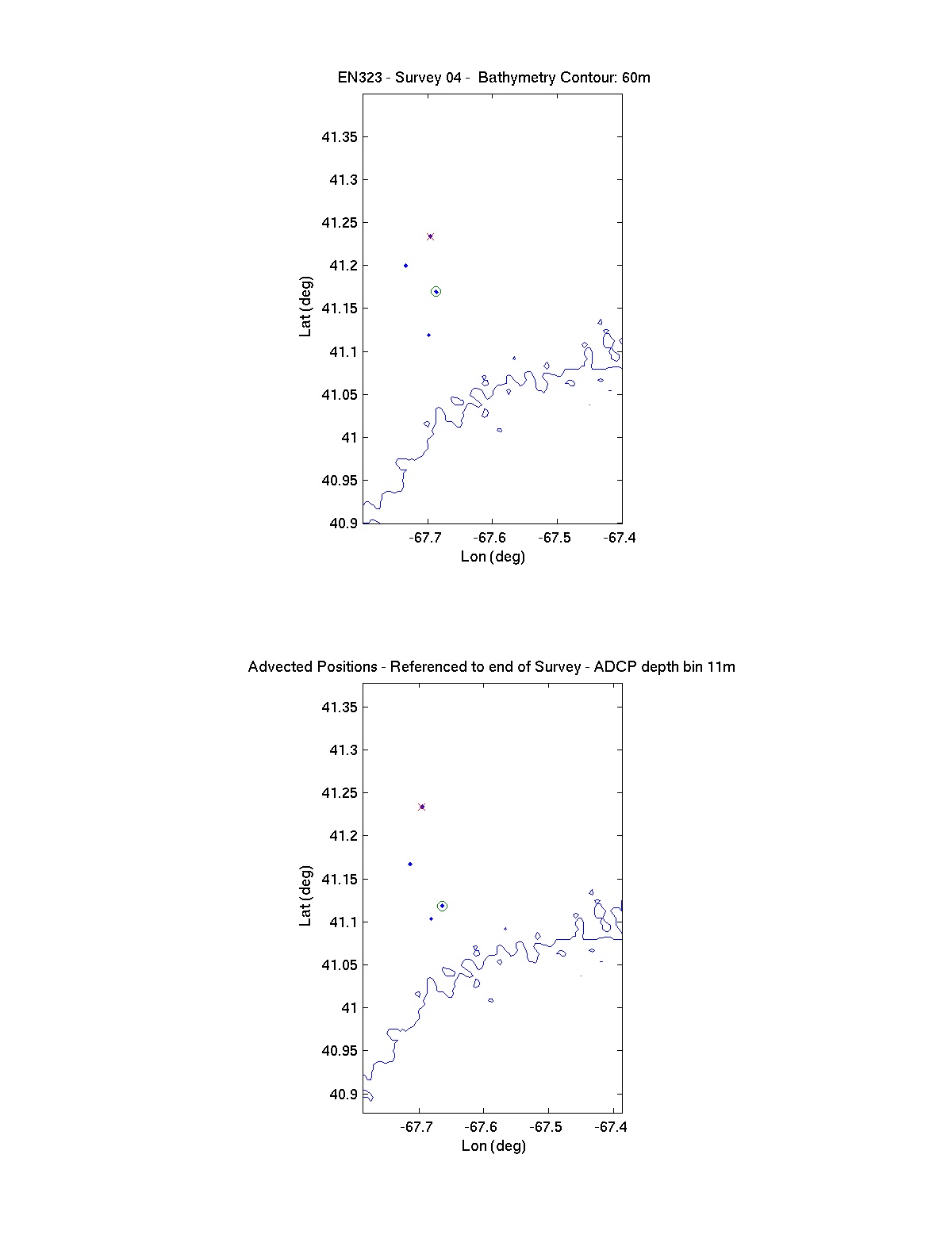
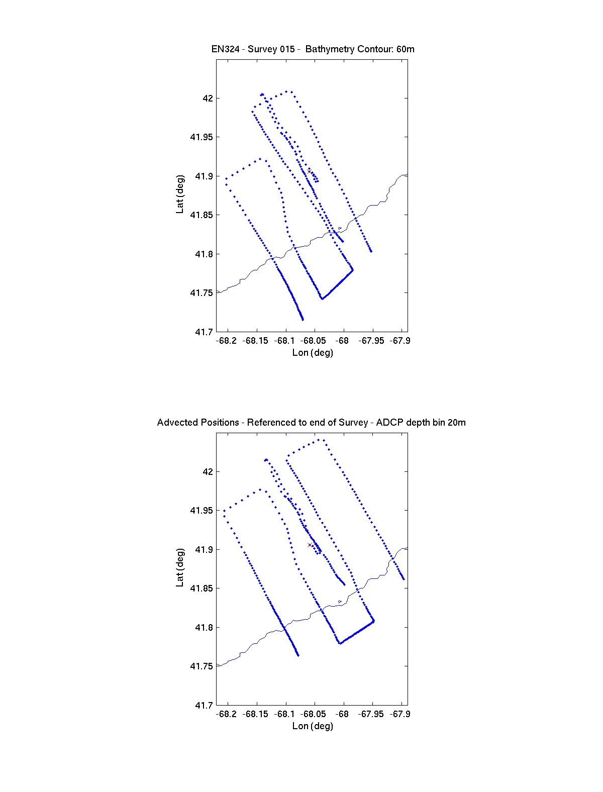
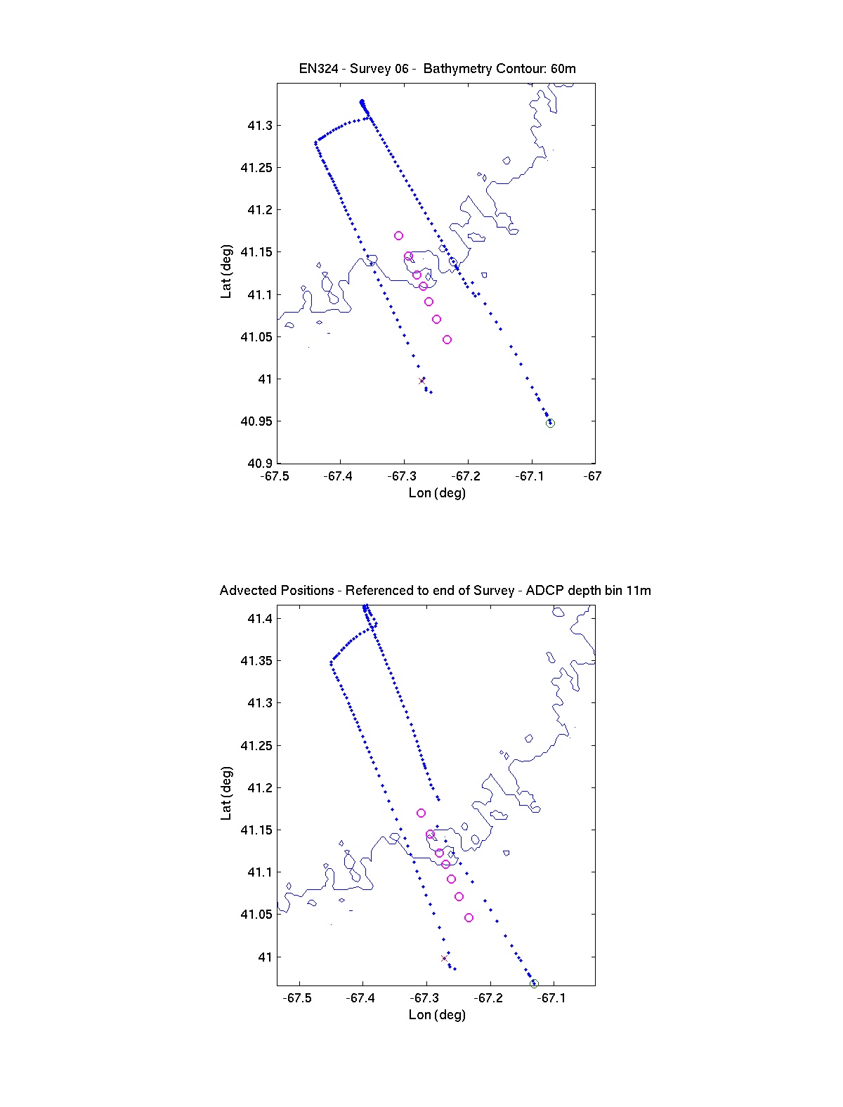
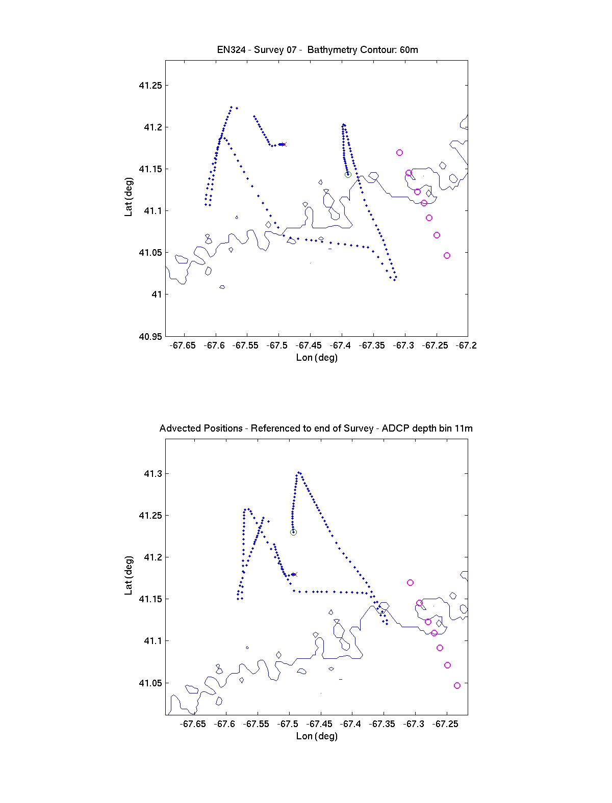
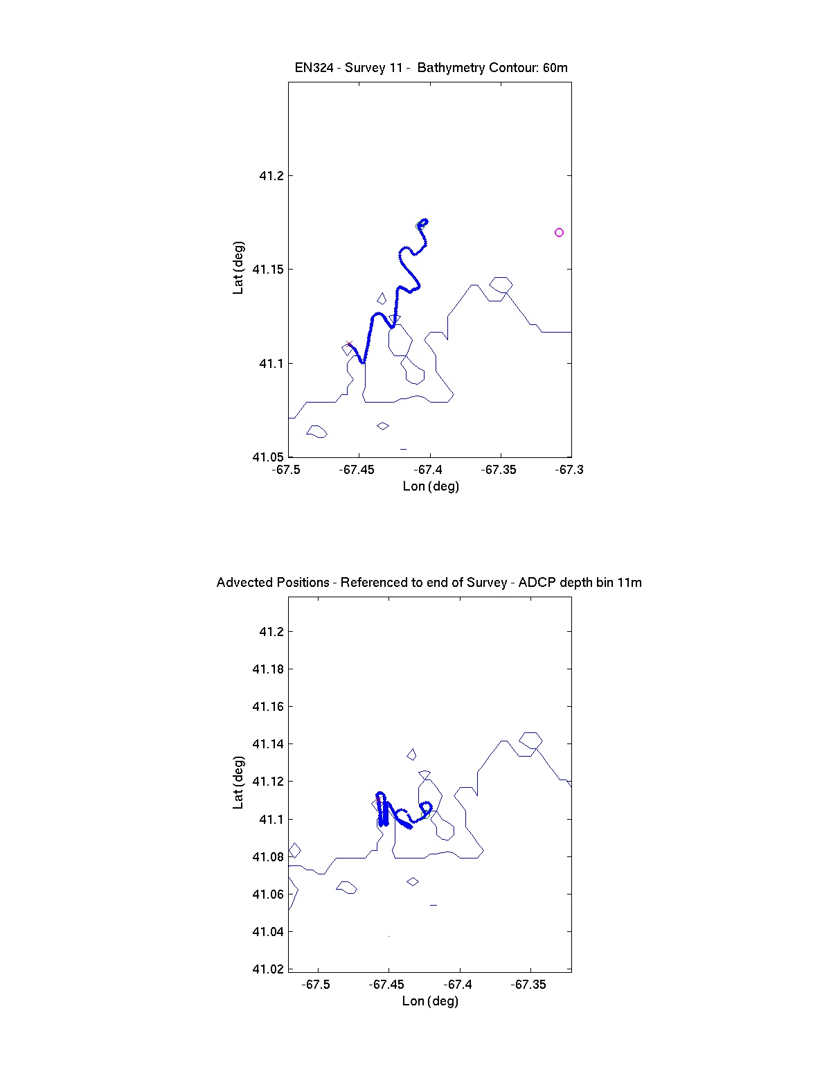
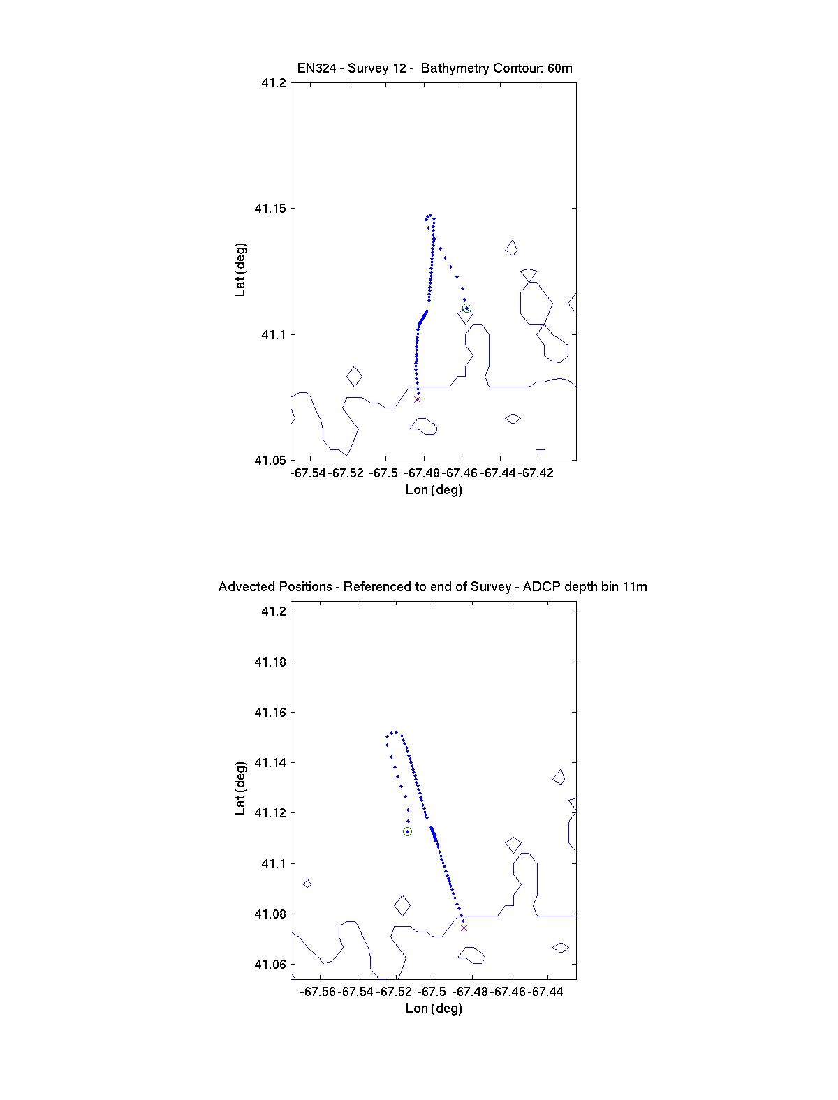
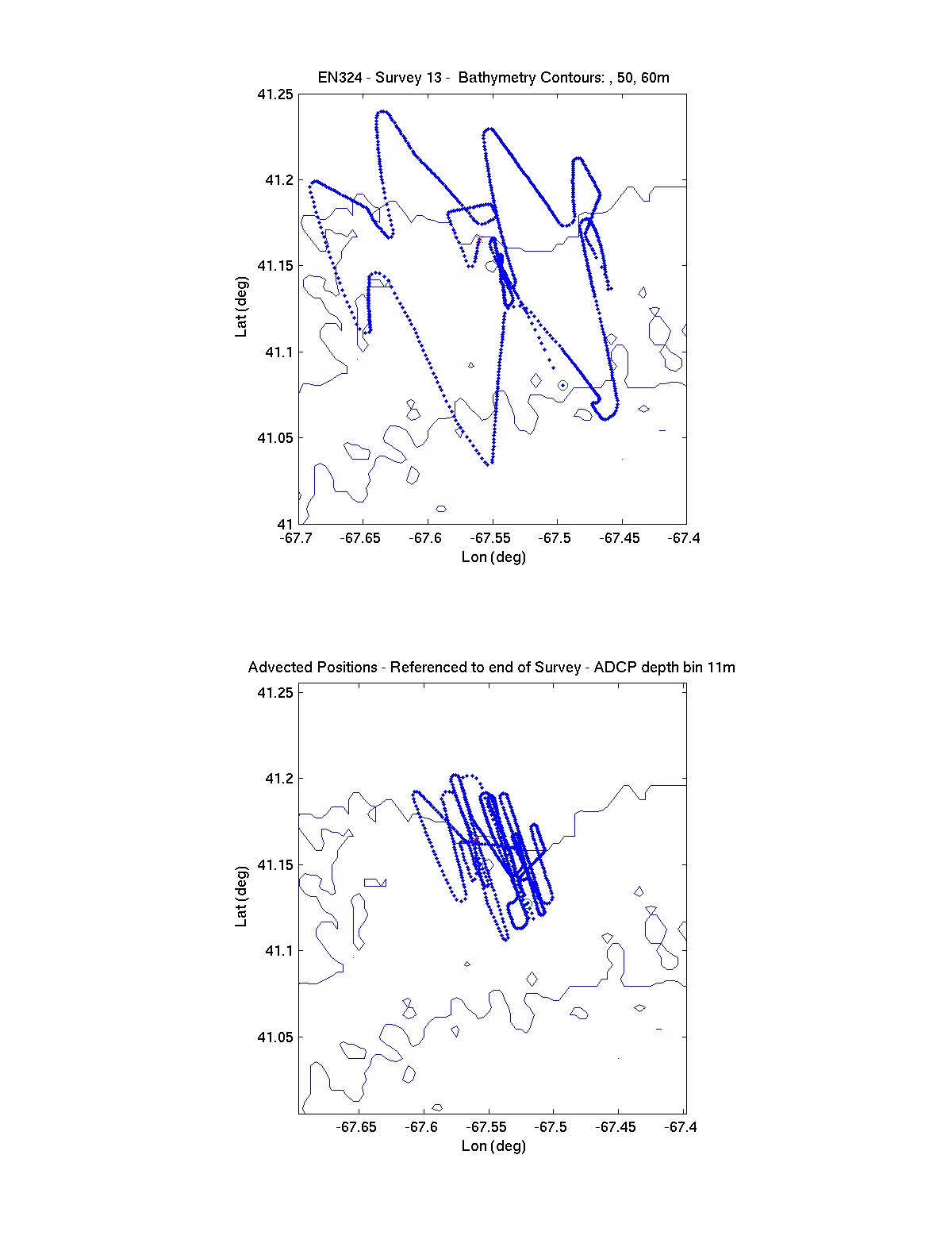
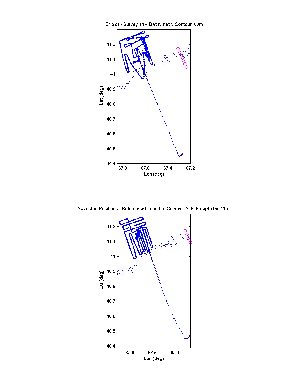
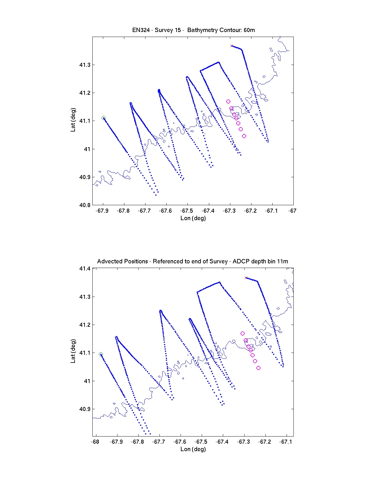
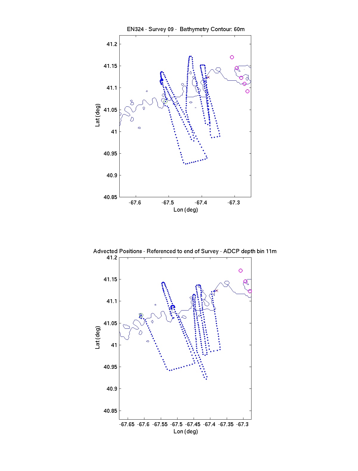
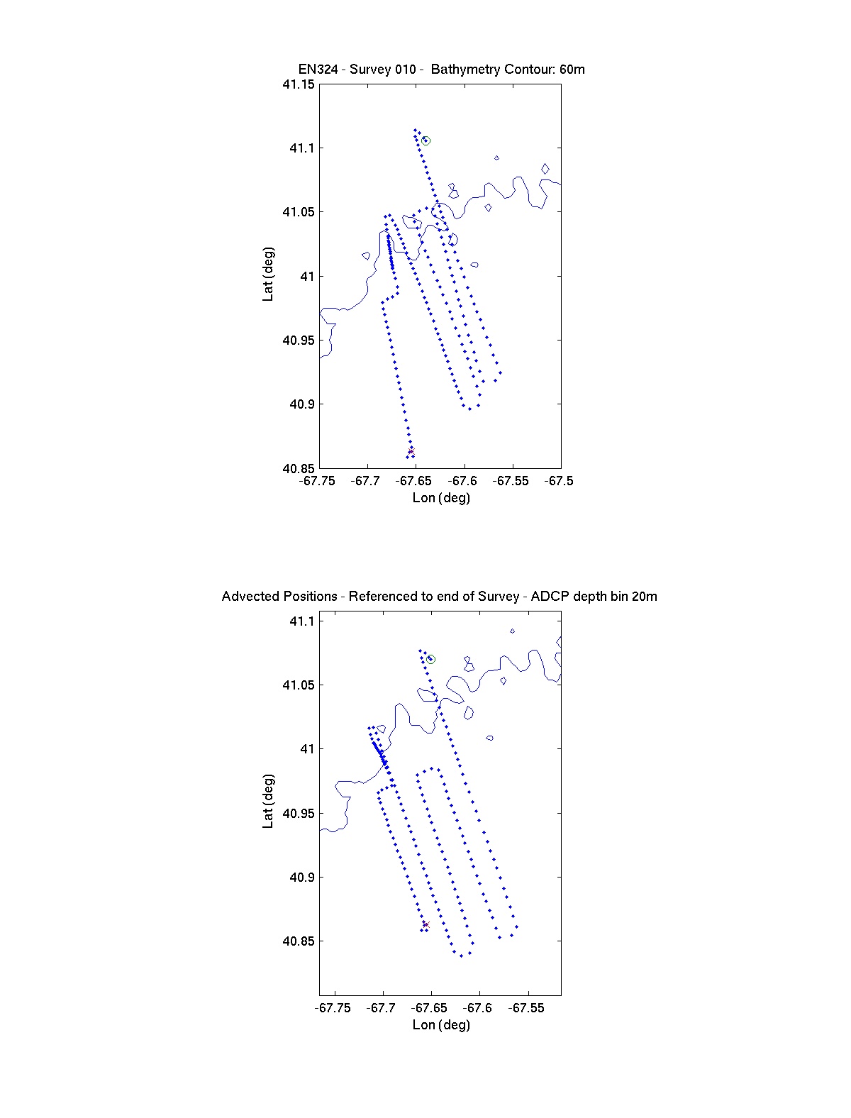
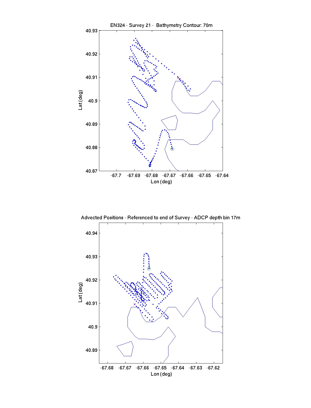
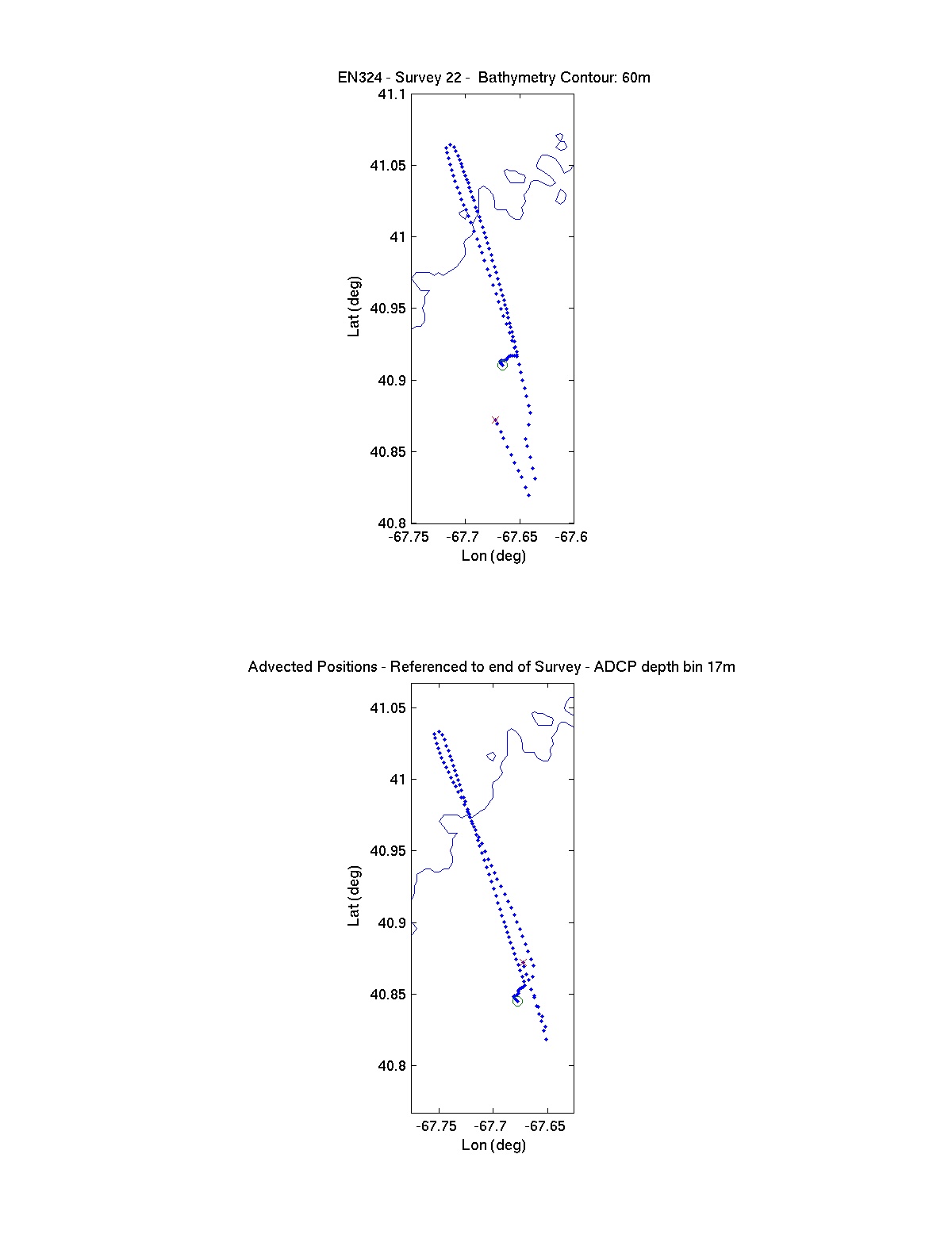
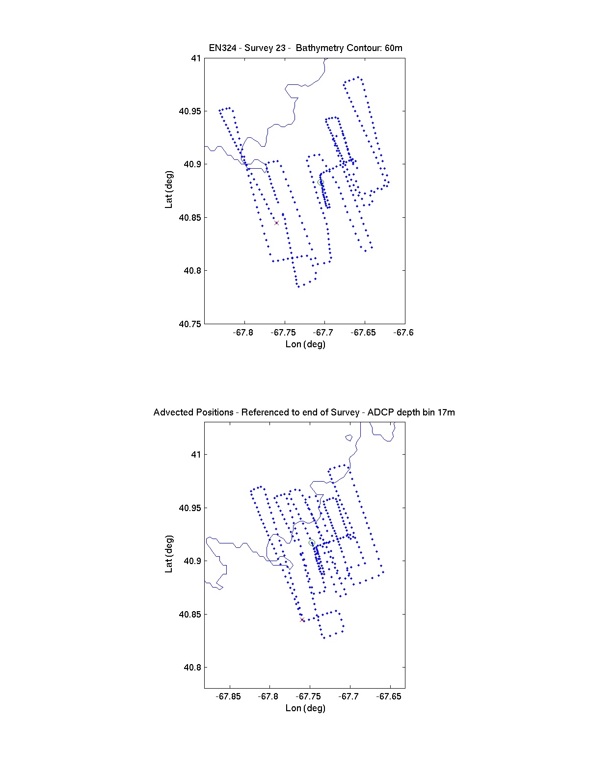
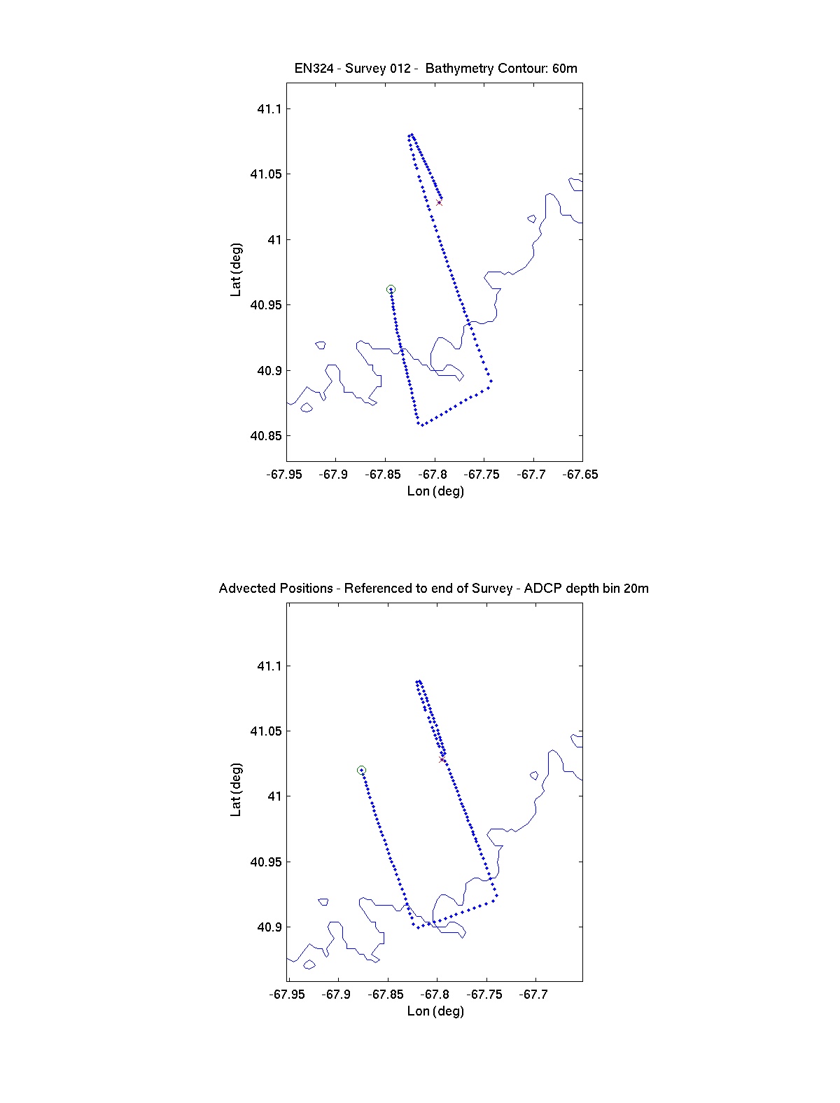
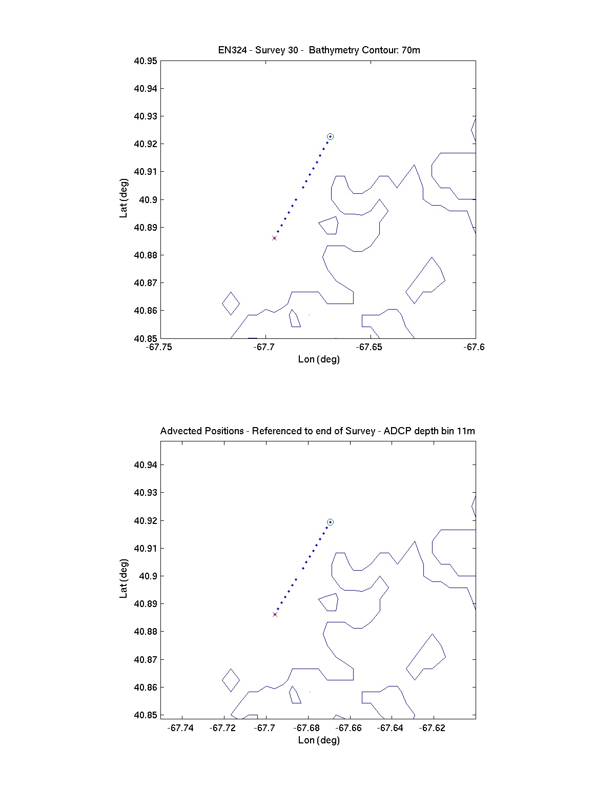
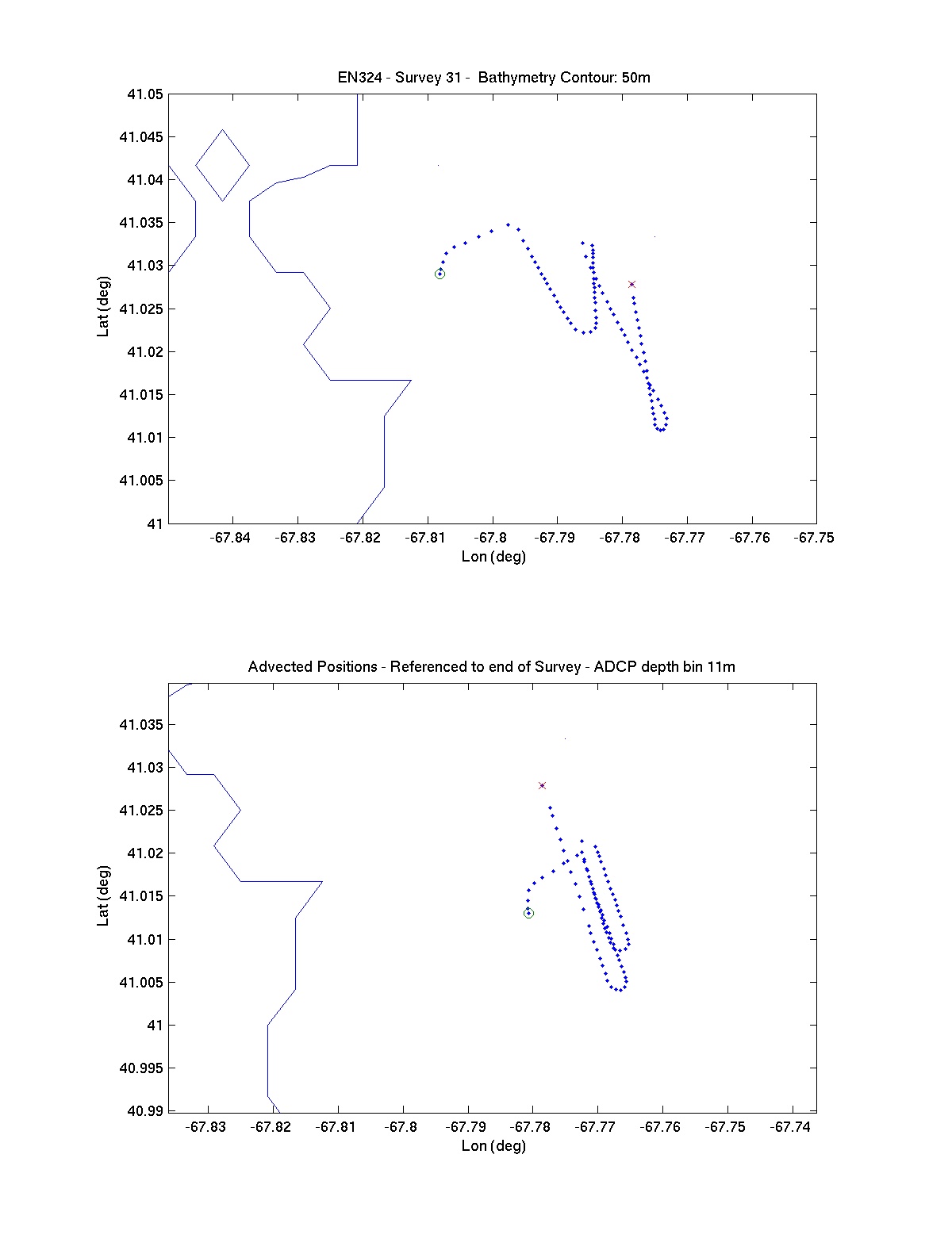
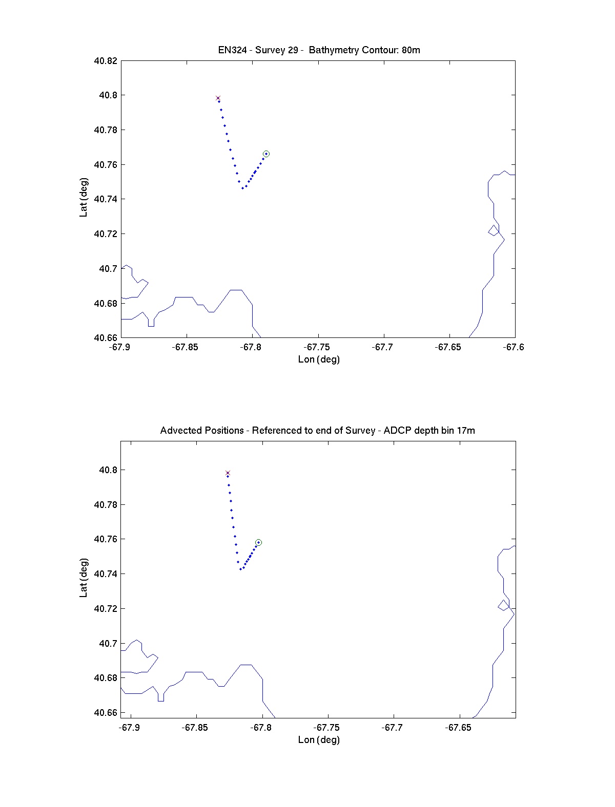
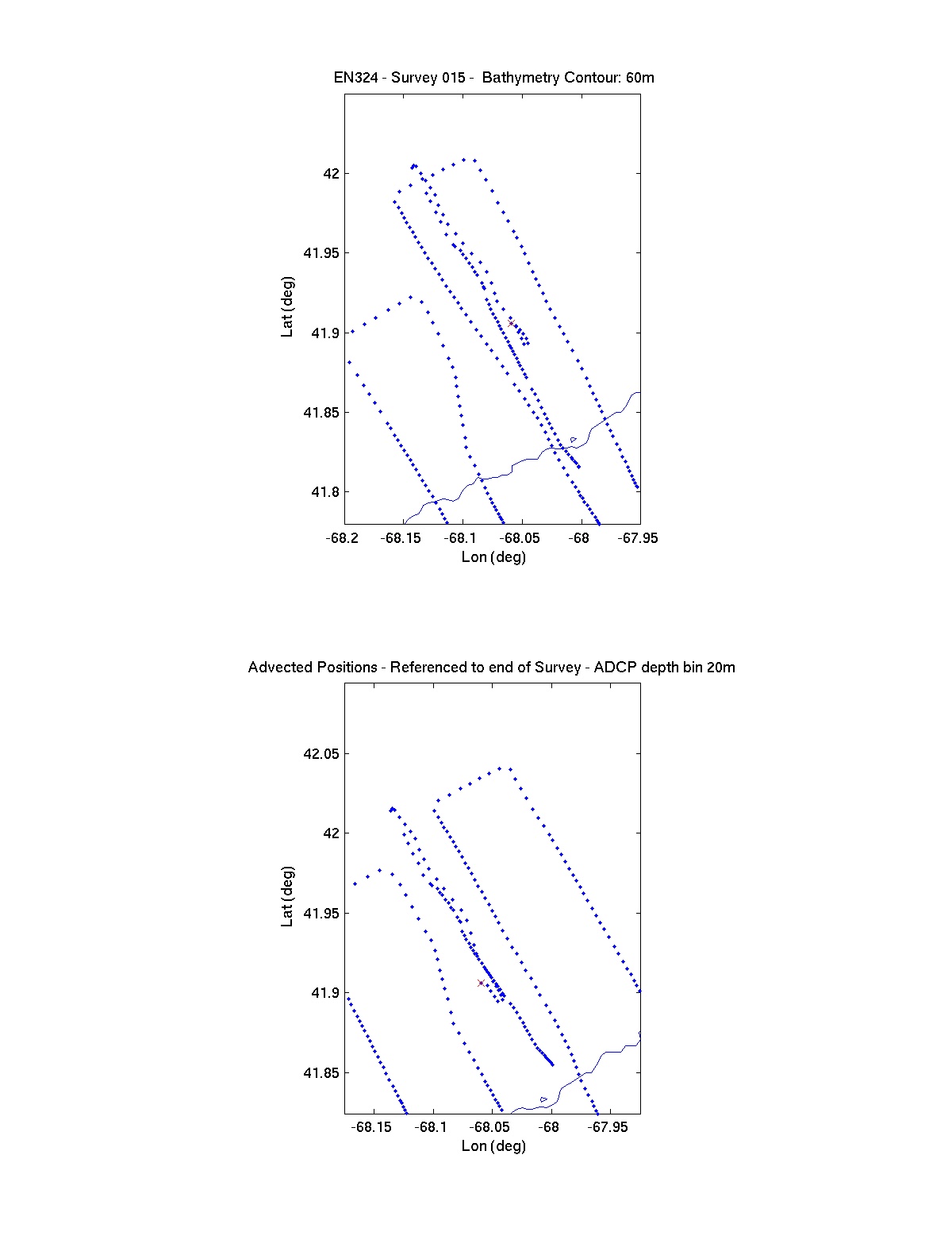
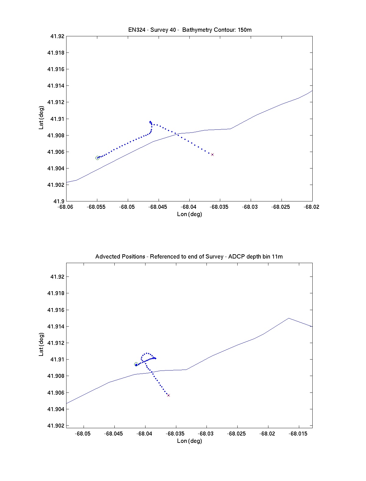
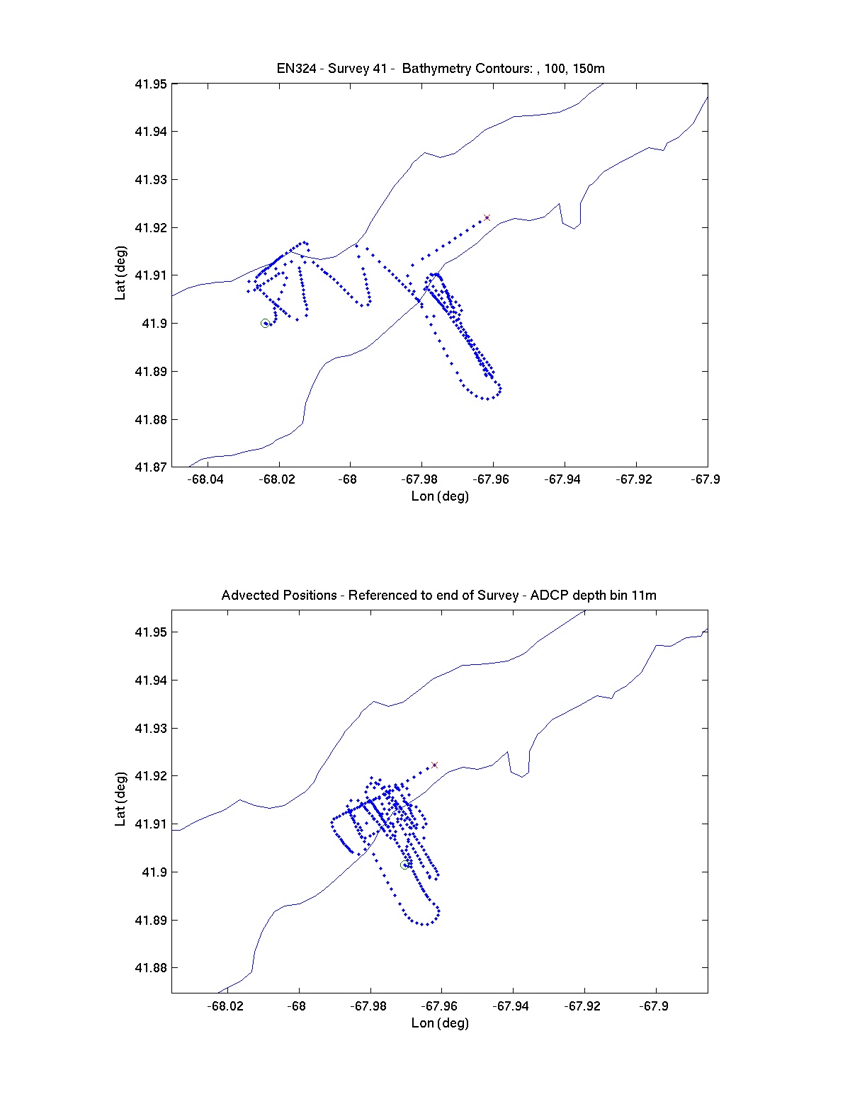
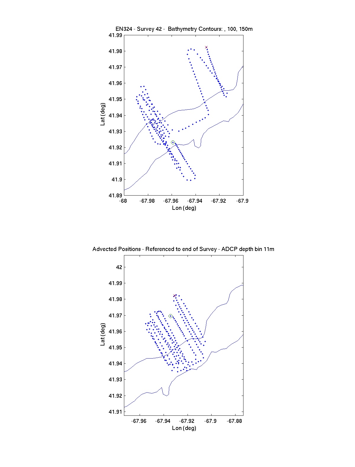
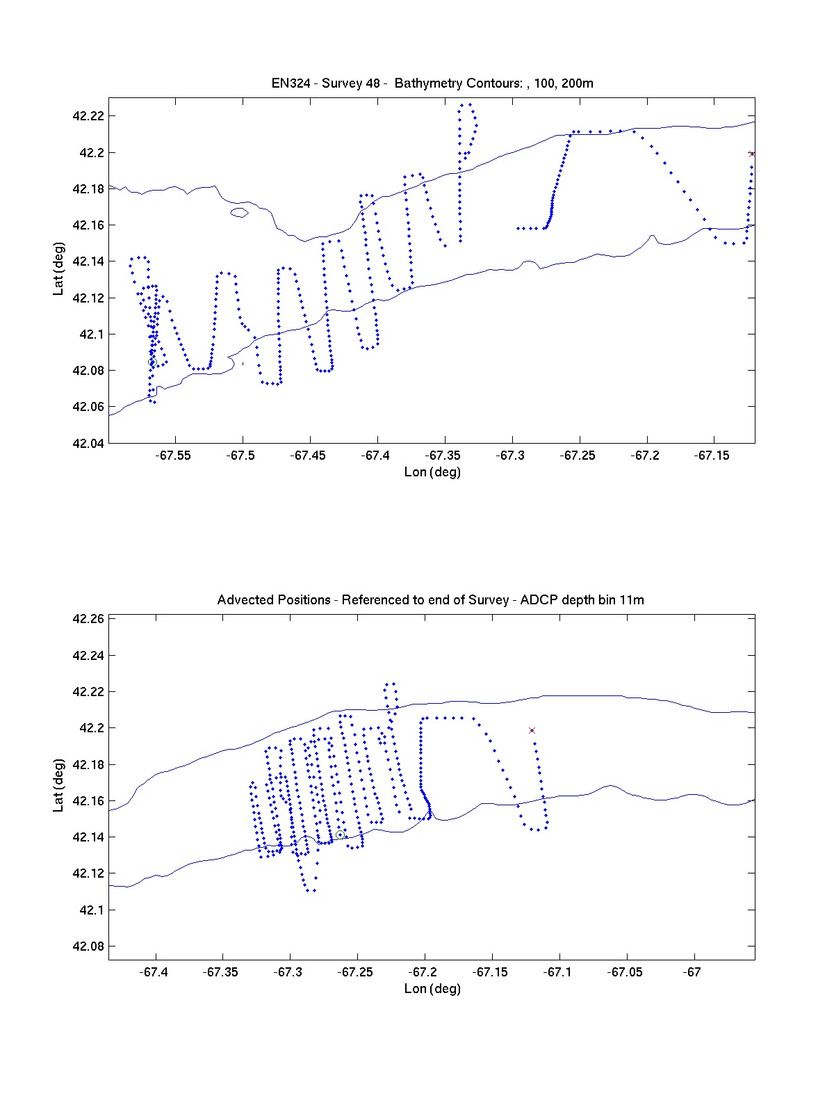
The dye was sampled with a Chelsea Instruments Aquatracka fluorometer mounted on the VPR tow vehicle, with the signal integrated with the VPR data stream. The fluorometers were calibrated on board using seawater from the site (Appendix 10.2). The data stream from the towed vehicle also included conductivity, temperature, pressure and chlorophyl measurements. The dye patches were tracked by integrating the ADCP velocities in the depth bin closest to the isopycnal surface of the dye release. These integrated velocities were also used to adjust the cruise track to make a sampling pattern that was reasonably well spaced in a reference frame moving with the water. Navigation was relatively easy in this region of strong, nearly barotropic tides. Straight lines relative to the moving water could be executed simply by holding the ship's heading constant, and ignoring earth bound coordinates. At times, windage required an adjustment of 5 or 10 degrees in heading to obtain the desired course through the water. The effectiveness of this method can be seen by comparing the upper and lower sampling traces shown in Appendix 10.6.
The ship's speed during sampling varied between 2 and 8 knots, slower speeds being used early in an experiment and 8 knots being used only for broadscale surveys. The winch speed for the tow-yos was 20 to 40 m/minute, with the towed body coming within 3 m of the surface and descending to 10 to 20 m above the bottom. The lateral resolution can be seen in the ship tracks in Appendix 10.6.
Analysis of the dye and hydrographic data required correction for background fluorescence and also for lags between the different sensors to obtain the most accurate estimates of the distribution of dye in density space. A preliminary look at the lateral distribution of the dye for the experiment in the pycnocline on the south flank is shown in Figure 4.1, which shows maps of the column integral of dye at 4, 41 and 117 hours after release. One can see that the main advection was along isobaths, while the patch spread strongly both along and across isobaths, i.e., toward and away from the tidal mixing front near the 60-meter isobath.
The locator map shows the dye release spot and the survey areas, with isobaths at 40, 60, 80, 100, and 120 m. The detailed figure shows the dye patch at the time of injection and the boxes are approximately 4, 41, and 117 hours after release. The contour labels in the 117-hour map are in kg/km^2. A high signal near the 60 m isobath, judged to be false, has been removed from this map. The stations and the maps have been translated to the position they would have at a single time using velocity data from the shipboard ADCP. The time chosen was at a time of maximum off-bank displacement in the semidiurnal tidal cycle in each case. The position of the front was near the 60-meter isobath. While measurement of motion of the center of mass relative to this front must await further analysis, eddy diffusion appears to have spread the patch both toward and away from the front.
James H. Churchill and Daniel J. Torres
Description
If classified by their current following properties, the drifters used in this study may be split into two categories: surface followers, and subsurface following, drogued drifters. The surface followers (hereafter, surface drifters) were rigged as "Davis-style" drifters. Their water drag was supplied principally by four nylon "sails" that radiated, in a cross-vane pattern, from the drifter's electronics canister. The sails were suspended between nylon rods, which extended through holes at the top and bottom of each canister. Buoying the drifter were four Styrofoam floats attached to the ends of the top rods. Each of the surface drifters was outfitted with GPS and ARGOS antennae, extending from the canister's top. Each drifter extended to roughly 1 m beneath the sea surface. All of the surface drifters were manufactured by Brightwater Instrument Corp.
Each drogued drifter was comprised of three components connected by tether lines. At one end was a surface electronics package, housed either in a buoyant sphere or in a canister buoyed by Styrofoam floats. This was horizontally tethered to a surface float, which was vertically tethered to a cylindrical drogue. Each drogue was roughly 6 m long by 1.6 m in diameter and supplied a minimum 40:1 drag ratio. Brightwater supplied most of the drogued drifters (these had canister-housed electronics). Three were purchased from MetOcean (these had spherical electronics housing).
Each drifter was outfitted with a near-surface thermistor, contained within the electronics housing. To obtain sub-surface temperatures from drogued drifters, we attached a self-contained, recording thermistor (manufactured by VEMCO Inc.) to the tops of most drogues. All drifters were also equipped with GPS electronics, for positioning, and with an ARGOS-PTT (VHF transmitter). Each PTT transmitted messages, with the GPS positions encoded, to ARGOS satellites. These messages were, in turn, relayed by System ARGOS, in e-mail correspondence, to the Endeavor twice a day. The ARGOS messages were also directly received aboard the Endeavor, when the ship was in VHF range of a drifter. These were decoded as part of real-time drifter tracking operations.
The only serious problem with using ARGOS for position transmission arose from the temporal spottiness of the ARGOS satellite reception. Typically, GPS positions were acquired every 20 min. For this rate, each ARGOS message should have contained positions acquired over the previous 5-6 hours. This would have been sufficient to transmit nearly all of the positions, in spite of gaps in the ARGOS reception due to absence of satellites in sky view. However, the drifters' transmission to the satellites was apparently not perfect. As a result, the GPS position records obtained from the ARGOS messages often contained daily gaps of 3 hr or more.
Aside from this problem, we were blessed with extremely good luck in our drifter operations, especially in drifter recovery. We considered the MetOcean units expendable and made no effort to recover these. The Brightwater's units were classed as reusable, and most were outfitted with strobe lights to aid in night-time recovery. All Brightwater drifters were eventually recovered and returned to WHOI.
Summary
During the cruise, we conducted five separate drifter deployments. Three were done in conjunction with dye tracking experiments, while the other two were done in preparation of a dye release. Summarized below are some preliminary findings from the drifter tracking. Presented as part of this are drifter tracks of each deployment (Figures 5.1-5). For clarity, not all drifter tracks are shown. For deployment #1, only the high-tide drifter positions are shown (determining high tide position for other deployments was precluded by the ARGOS dropout).
Table 5.1 - Summary of Drifter Deployment/Recovery Locations and Times for EN323/4
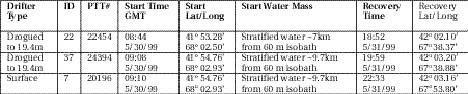
5.1a. Deployment #1 - Southern Flank
5.1b. Deployment #2 - with the Southern Flank Surface Dye Release
5.1c. Deployment #3 - with the Southern Flank Pycnocline Dye Releases
5.1d. Deployment #4 - Northern Flank
5.1e. Deployment #5 - with the Northern Flank Pycnocline Dye Release
**Drifter 37 was initially deployed with Drifter 7 near the center of the dye patch during injection. However, its power connector disconnected upon impact with the water. It was recovered at 41° 54.01' /67° 58.18, repaired and redeployed at the location shown above.
Deployment #1 - May 7-10
In this first drifter study, conducted as a prelude to the Southern Flank dye tracking experiments, we sought to explore convergence onto the tidal mixing front from both the stratified and unstratified regions. Drifters were placed on either side of the front and within the frontal region (Table 5.1a). A surface and drogued drifter were placed in stratified water within a few hundred meters of the front. These were flanked by a surface drifter set out in unstratified water ~8 km NNW of the front, and by a drogued and surface drifter pair set out in stratified water 7 km SSW of the front. All of the drogues were set at a mean depth of 19.4 m, roughly the center depth of the pycnocline as it appeared in the CTD data acquired before the drifter deployment.
Unfortunately, the surface drifter set out at the front, #8, only transmitted once after being released. The tracks of the other drifters revealed a clear difference between the surface and pycnocline flows in the stratified water south of the front. As evidenced by their high-tide positions (Figure 5.1), the surface drifters moved onbank, to the northeast, over the first 4-5 tidal cycles. They were likely carried by a wind-driven surface flow. The wind was to the west, downwelling favorable, over the first 2.5 days of the deployment and had a strong northward component between deployment days 1.5 and 2.5. The drogued drifters showed a clear onbank variation in the along-isobath flow. The drogued drifter set out near the front traveled westward roughly along the isobaths. Over the first two tidal cycles, it translated westward at a mean speed of roughly 8 cm/s. The drogued drifter deployed south of the front made little progress in any direction. As indicated by its surface and sub-surface T-pod temperatures, it remained in stratified water. However, both the drogued frontal drifter, and the surface drifter deployed south of the front made their way to the well mixed zone, as indicated by the convergence of their surface temperatures with the surface temperatures measured by the drifter deployed in mixed zone. Taken together, the tracks and temperatures of the drifters suggested a convergence of near-surface flow onto a strong along-isobath flow at the tidal mixing front.
Figure 5.1. "High tide" positions (maximum northward tidal excursions) of the drifters set out over the southern flank on 7 May 1999. Crosses mark the high tide locations. The start and end of each track are marked by a square and circle, respectively. The magenta contour depicts the 60 m isobath.
Deployment #2 - May 16-19
The second drifter deployment was done in conjunction with the Southern Flank surface dye experiment. A total of six surface drifters were set out (Table 5.1b). The first was deployed near the tidal mixing front prior to the dye injection. Dye injection into the surface mixed layer commenced roughly 1.5 hr after the release of this drifter. The injection site was roughly 5.5 km SSE (~2.4 km east and 4.9 km south) of the drifter's position. Three drifters were deployed within the dye patch, with deployments occurring after the injection of 1, 2 and 3 (out of four) barrels of dye. Roughly five hours after the dye release (following the first dye survey) a drifter was placed between the dye and the front. An hour later, the final drifter was set out ~2 km to the south of the dye patch.
The drifter thermistor records indicated that all drifters were carried to the tidal mixing front. All moved to 8 °C water (presumably the temperature of the mixed zone) within two days after release. This was likely due to forcing of the surface layer by the local winds, which were directed to the northwest (downwelling favorable) throughout the deployment. The subtidal motions (Figure 5.2) of all drifters deployed south of the front were remarkably similar. All of these drifters moved at about 14 cm/s westward and 4.5 cm/s northward over the first two days, and at about 5 cm/s westward and 3 cm/s southward over the final 1.5 days. This slowing of the drifters was not matched by an appreciable decline or direction shift in the wind recorded at buoy 44011. The frontal drifter moved slightly more slowly to the west but somewhat more rapidly in the northward direction (at about 6 cm/s over the first two days).

Figure 5.2. Tracks of three of the six surface drifters deployed on 16 May 1999 in conjunction with the Southern Flank surface dye experiment. Boxes mark the deployment locations, and the legend describes these locations.
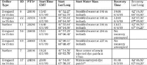
Deployment #3 - May 23-28
This deployment was done as part of the 1st pycnocline dye injection. A total of seven drifters were deployed (Table 5.1c). The first was a surface drifter set out in slightly stratified water (8.8 °C at 1m and 7.4 °C at 5m) near the front. The dye release commenced roughly 2.5 hrs later and roughly 16 km to the SE of the drifter. Four drifters were released during dye injection. Drifters drogued at 19.4 m were set out after 1, 2 and 3 barrels of dye, and a surface drifter was set out after 3 (of 3 total) barrels. Two additional drifters were deployed after the first dye survey. One was a "subpycnocline" drifter set out at the dye patch. Its drogue was set at a mean depth of 39.4 m, and was most likely always in the well mixed layer beneath the pycnocline. The other was a "pycnocline" drifter (drogued to 19.5 m mean depth) released about 3 km to the south of the dye patch.
The drifter tracks (Figure 5.3) showed a clear depth and horizontal variation of the subtidal flows within the stratified region. The surface drifter deployed over the dye patch initially moved northeastward to the roughly 60-m isobath. Thereafter, it apparently "stalled", having little net subtidal displacement. In marked contrast, the surface drifter deployed near the front steadily moved to the northwest throughout the deployment. A likely explanation for this behavior is that the dye patch surface drifter encountered a zone of convergence at or near the front, while the frontal drifter moved into the mixed zone early in the deployment and was carried, unfettered, by the wind-driven near-surface flow.
Figure 5.3. Tracks of four of the seven drifters deployed on 23-24 May 1999 in conjunction with the first Southern Flank pycnocline dye release. Boxes mark the deployment locations, and the legend describes these locations.
In contrast to the surface drifters, the pcynocline drifters moved westward. Tracks of pycnocline dye drifters (Figure 5.3) offer some evidence that they were carried onbank to a zone of relatively strong along isobath flow. Over the first four tidal cycles, they moved at about 4 cm/s to the WNW (1 cm/s to the north and 4 cm/s to the west). Their speed was significantly greater, about 7.5 cm/s to the WSW (3.5 cm/s to the south and 6.5 cm/s to the west), over the next 6 tidal cycles. The pycnocline drifter deployed south of the dye patch also experienced an acceleration (although smaller) to the WSW. The subpcynocline drifter was apparently carried by a slightly different flow than its pcynocline counterparts, with a higher southward but smaller westward component. Conclusions drawn from a comparison of the drifter tracks must be qualified, however, because of differences in the setups of the drifters. The pcynocline drifters had a larger electronics package than the subpycnocline drifter.
Deployment #4 - May 30-31
This deployment was done to sample flow over the slope off the Northern Flank in preparation for the Northern Flank dye experiment. Three drifters were released (Table 5.1d). A drogued drifter was set out over the 110 m isobath (~7 km north of the 60 m isobath), and a surface and drogued drifter pair were deployed about 2.7 km further north over the 167 m isobath. Both drogued drifters were rigged to give a 19.4 m mean drogue depth. Tracks of the two drogued drifters (Figure 5.4) revealed a strong pycnocline flow which carried water towards the Bank. Estimated subtidal velocities of these drifters were 30 cm/s alongslope and 2 cm/s onslope (toward the Bank). This strong current, moving onbank, apparently did not extend to the surface. The surface drifter moved offbank at a subtidal speed of roughly 13 cm/s. Although weak, the wind may have been partially responsible for the vertical shear observed by the drifters. Throughout the deployment, winds measured at buoy 44011 were directed northward with a magnitude of roughly 3 m/s.
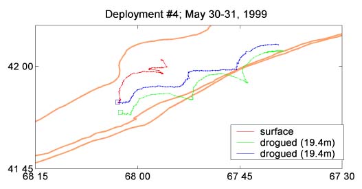
Figure 5.4. Tracks of the drifters deployed on 30 May 1999 in preparation for the Northern Flank dye release. The magenta contours depict the 60, 100 and 200 m isobaths.
Deployment #5 - June 1-6
This deployment was done as part of the Northern Flank dye experiment. Prior to the dye release, five drifters were deployed along a line extending NNW from the northern flank (Table 5.1e). Drifters drogued to 19.4 m were set out over the 100, 186, 204 and 227 m isobaths, and a surface drifter was released over the 186 m isobath. In addition, a surface and a 19.4 m drogued drifter were deployed within the dye patch. This was a deployment marked by a number of remarkable drifter "mishaps", which are described in the Cruise Narrative.
Tracks of the drogued drifters (Figure 5.5a) revealed two distinct current regimes off of the Northern Flank. The drogued drifters set out over the 100 and 186 m isobaths were carried rapidly to the NE by a strong along-bank current. Their tracks revealed a weakening of this current going away from the Bank. Over the first day, the drifter set out over the 186 m isobath traveled at a mean speed of ~20 cm/s (before its drogue tether was severed), whereas the drifter released at the 100 m isobath moved at a mean speed of ~27 cm/s. Tracks of the drogued drifters deployed further north revealed a rapid offbank transition from the strong northeastward flow over the upper slope to weak westward current over the lower slope. Over the first day, the drifter set out over the 204 m isobath traveled to the northeast at only 9 cm/s, while the drifter set out over the 227 m isobath traveled westward at ~7 cm/s. Eventually, both drifters were entrained in this westward flow.
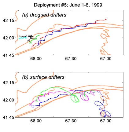
Figure 5.5. Tracks of the drogued (a) and surface (b) drifters deployed on 1 June 1999 in conjunction the Northern Flank dye release. The green colored track in both panels depicts the path of the same drifter, which was converted from a drogued to a surface drifter by a fisherman.
Comparison of the drogued drifter tracks from deployments 4 and 5 revealed a fairly rapid change in the cross-bank flow within the pycnocline off the Northern flank. The 2 cm/s onbank flow revealed by the tracks of the pycnocline drifters of deployment 4 played a large role in our choice of an outerslope dye release location (over the 170 m isobath). Unfortunately, this onbank flow had disappeared by deployment 5. Tracks of the pycnocline drifters of deployment 5 revealed an offbank flow over the upper and outer slope.
The cross-slope component of surface flow had also apparently changed in sign from deployment 4 to 5. The surface drifter set out in deployment 4 tended to move away from the bank, whereas all surface drifters released in deployment 5 were eventually carried onto the bank crest (Figures 5.4 and 5.5b).
The local winds may have played a role in the shift in cross-slope flow direction. Winds measured at buoy 44011 were light (<4 m/s) and directed to the NNE during deployment 4, but became stronger (>7 m/s) and shifted from northeastward to southeastward during deployment 5.
6. REAL-TIME DATA ASSIMILATIVE MODELING OF THE FLOW FIELD
Dennis McGillicuddy and Valery Kosnyrev
R/V Endeavor cruises EN323 and EN324 were part of the U.S. Globec Georges Bank Phase III study focused on cross-frontal exchange. The principal objective was simultaneous assessment of the transport of water and plankton in the vicinity of the tidal mixing front. The approach was to inject Rhodamine dye into specific density strata and then measure the movement of the dye patch and the associated planktonic community with respect to the neighboring front. This was accomplished through incorporation of the fluorometric dye detector into the Video Plankton Recorder system, facilitating real-time assessment of both tracer and plankton distributions (down to the species level). The adjacent waters were also seeded with radio- and satellite-tracked drifters. Real-time data assimilative modeling of the flow field (and associated transports of tracer and plankton) was carried out in concert with the observational activities, in order to (1) provide an additional interpretive framework for the measurements, and (2) provide nowcast/forecast products which could be used in planning sampling strategy.
This general experimental design was implemented in three different tracer injections:
(1) South Flank - surface
(2) South Flank - pycnocline
(3) North Flank - pycnocline
Observational and modeling activities for the first two were coordinated with the R/V Edwin Link, which also had a real-time modeling effort aboard. There was observational coordination with R/V Oceanus in the latter two experiments.
Details and further results from these studies are reported in McGillicuddy and Kosnyrev, 2000, U. S. Globec Data Report "Real-time Modeling on R/V ENDEAVOR Cruises 323 & 324 to Georges Bank: 5-12 May & 14 May- 7 June 1999."
Each of the three experiments was associated with distinct biological circumstances. During the surface dye experiment, Calanus was abundant in the stratified waters and nearly absent in the well-mixed area where hydroid predators were present in large numbers. Intensive survey operations revealed striking covariance in the fine scale distribution of these two animals. The South Flank pycnocline release was purposefully located in a patch of Calanus. As the dye patch was tracked over the following four days, Calanus all but disappeared from the tagged water mass. The decrease in Calanus abundance was accompanied by the appearance of large schools of herring, mackeral and whales which were observed feeding at the surface. Finally, the North Flank pycnocline experiment was carried out in the presence of very high concentrations of the colonial diatom Chaetoceros socialis. These phytoplankton were most abundant in a thin (~5m) layer at the base of the pycnocline in the stratified area, but their distribution clearly extended into the well mixed region.
The real-time modeling effort was focused on diagnosis and prediction of water movement and associated transports of tracer and plankton. A data assimilative regional circulation model was used to produce hindcasts, nowcasts, forecasts from which the relevant transports could be gleaned. Skill of the model predictions was evaluated against observed drifter trajectories. On the basis of those assessments, the best forecast runs were selected for use in operational products supplied to the chief scientist. These products took several forms: (1) "stick plots" of the modeled velocity at a particular site [for planning tracer injections with the phase of the tide], (2) time-annotated trajectories of both fixed-depth and fluid following particles (representing drifters and dye, respectively), (3) animations of clouds of fluid-following particles (representing dye), and (4) synoptic maps of the dye observations generated by advecting the station locations with the model flow field. In addition to these operational products, model solutions were also used as a basis for data-assimilative coupled physical/biological simulations. Observed distributions of Calanus and hydroids were assimilated into the modeled flow fields in order to assess their relative transports and interactions.
In all, 170 model simulations were carried out during the two cruises, consisting of hindcasts, forecasts, sensitivity analyses and coupled physical/biological runs. This archive of model calculations and observations provides a basis for evaluating the performance of the forecast system, and determining under what conditions it performs best. Generally speaking, model forecasts were improved most by (1) using the most recent hydrographic observations for prescribing the mass fields used in the initial condition; (2) forcing the model with observed winds for that portion of the simulation which precedes bell time; (3) assimilating the "right" amount of ADCP data. This final point requires explanation. During some periods of the experimental work, forecast skill was consistently improved by adding more observations. However, such was not always the case, particularly on the North Flank. Apparently there was significant time-dependence in the flow, for which the best treatment in the current forecast system was careful temporal windowing of the ADCP data which were assimilated. Explicit representation of this time dependence is a recommended avenue for further research.
In aggregate, the error growth characteristics of the model forecasts were surprisingly uniform. For the four-day time horizon over which forecast skill was evaluated in the various experiments, forecast error was a linear function of the duration of the prediction (Figure 6.1). On average, separation between simulated and observed trajectories of drifters and dye grew at a rate of 3 km/day. This is a remarkable statistic given that the RMS error of the model fit to the ADCP data rarely fell below 7 cm/sec, and was commonly in excess of 10 cm/sec. Furthermore, the relative uniformity of the growth rate over such a wide range of conditions is worthy of note.
There are several opportunities for further improvement of the simulations in a hindcast mode. For example, additional observations can be assimilated, such as the drifter data themselves (these data were used for forecast evaluation and therefore not assimilated) and mooring records (not available in real time). Synthesis of all available observations in the context of hindcast simulations will provide realistic representation of the three-dimensional physical and biological fields as they evolve in time. These space-time continuous fields will be used to diagnose the underlying physical and biological processes involved in cross-frontal exchange on Georges Bank.
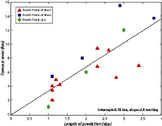
Figure 6.1. Forecast error (measured as the distance between simulated and observed trajectories of dye/drifters at the end of the data record) plotted as a function of the duration of the prediction. Each point represents the best forecast for each skill evaluation conducted during cruises EN323 and EN324.
7. VIDEO PLANKTON RECORDER (VPR)
Cabell S. Davis, Scott M. Gallager, Carin J. Ashjian, Andrew P. Girard, Philip Alatalo, and Qiao Hu
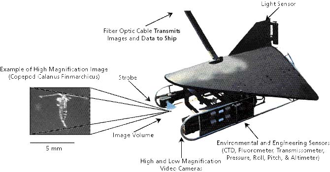
Figure 7.1. Schematic of the towed Video Plankton Recorder System as used on the cruise.
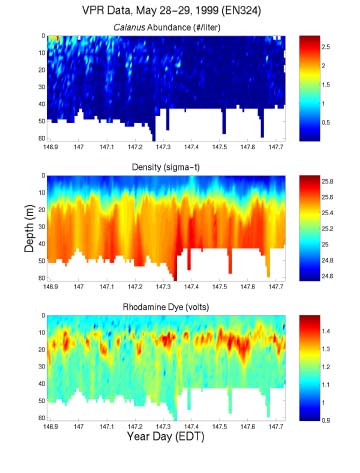
Figure 7.2. Panel color contour plot of Calanus abundance, sigma-t, and rhodamine concentration versus depth and time. These data are from a vpr tow made in a patch of Calanus and dye over about a 22 hour period on May 28-29 on the south flank. The dye had been released in the pycnocline. The figure shows how the Calanus disappear while sigma-t and dye remain unchanged.
Scott M. Gallager, Andrew P. Girard, and Philip Alatalo
Sampling Objectives
The objectives of this component of the cruise were:
1) To use the WHOI Sea Rover ROV and our 3-D plankton imaging system on Georges Bank to observe and quantify plankton motion vectors as a function of position in the tidal mixing front, tidal phase, prevailing hydrographic characteristics, biological communities, and light conditions.
2) To incorporate taxon-specific data obtained in Objective 1 into numerical models describing plankton distributions, residence times, and transport rates in relation to the observed behavioral responses.
The focus for Phase III of the U.S. GLOBEC Georges Bank Program is to determine the impact of frontal systems on controlling transport of plankton populations within and around Georges Bank. During EN323/324, the microscale to mesoscale distribution of plankton in relation to the tidal mixing front located at the 60 m isobath was studied in detail using the towed Video Plankton Recorder (VPR). Simultaneously, Lagrangian descriptions of water mass transport were studied using passive dye as a tracer, drifters, and the shipboard ADCP. The study of plankton motion vectors was undertaken to allow direct quantification of plankton behavior for incorporation into the plankton transport models.
Hypothesis
Based on the general observation of negative phototaxis and positive rheotaxis in zooplankton, our three-step hypothesis regarding plankton patch formation and transport in tidal mixing fronts on Georges Bank is as follows: First, animals swim vertically to an interface (surface) greatly increasing their concentrations by moving essentially from a 3-D distribution toward a 2-D distribution. Second, upward swimming in combination with down-welling in a convergence zone will further increase zooplankton abundance as the animals move from a 2-D to a 1-D distribution. Third, once concentrations reach a critical level such that the nearest neighbor distances bring individuals within their perceptive distance, dense aggregations will form for the purpose of mating, feeding and predator avoidance. The basis of this hypothesis rests on the need for zooplankton behavior to be well structured and consistent within a population; However, we have no information on the level of individual variation in response to environmental conditions and what that variation means to a population's distribution.
Methods and Results
The WHOI Sea Rover ROV was fit with a 3-D imaging system designed to image plankton in their natural state. Two video cameras with appropriate lenses to provide a field of view of 35x 30 mm were positioned orthogonally on an aluminum frame extending 1.5 m in front of the ROV (Fig 8.1). Two 20 w xenon strobes filtered to a wavelength of >650 nm were synchronized with the video signal and positioned 8 degrees off-axis of each camera to provide a dark field, forward scattered imaged.

Figure 8.1. Photograph of SeaRover with 3D imaging system mounted on front. The imaging system consisted of two cameras and two strobes mounted such that XY and YZ coordinates could be extracted directly from the images. The imaging volume was 3.5x3.0x3.5 cm or 36.75 ml imaged at a rate of 60 Hz. Video signals were sent directly to a RGB frame grabber where the two signals were combined into a single image for later decomposition and processing. The ROV maneuvered well even with the camera frame hanging off the front. The main limitation to extended viewing of plankton was length of the tether which tugged on the ROV as the ship swung on its axis.
Sampling Strategy
The sampling strategy was to deploy the ROV and profile down to its maximum depth of about 50 m then return to the position in the water column where plankton were most abundant (Fig 8.2). The latter was always in the region of or just above the thermocline at a depth of about 10 m. We attempted to deploy at three locations normal to the front; However, this was not always possible to due to weather and sampling priorities. The ROV and 100 m tether were deployed from starboard midships using the J-frame. The distal 50 m of tether was made near neutrally buoyant using small plastic floats while the proximal 50 m was floated on the surface. This effectively decoupled ship motion from the ROV when it was at depth between 5 and 20 m, but did little to help translation of motion at depths greater than 20 m when the tether was taught or under the effect of surge near the surface. Once in the region of greatest abundance, the ROV moved slowly forward attempting not to disturb the flow. The 50 m of neutrally buoyant tether severely limited travel away from the vessel particularly as the vessel swung on its axis using the bow thruster in an attempt to maintain heading. In general the conclusion was that ROV ops were severely affected above a wind speed of 15 kts and impossible above 20 kts. To maximize sampling time and data quality, it is recommended that a ship with dynamic positioning capabilities be used in future ROV operations.
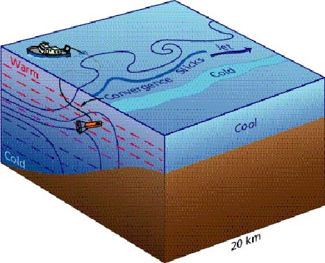
Figure 8.2. Cartoon of the deployment scheme used for the ROV and 3D imaging system along the 60 m isobath at the tidal mixing front on the Southern Flank of Georges Bank. Solid lines with arrows indicate secondary circulation associated with convergence zone where we observe plankton to concentrate. Dotted lines are the ROV survey tracks. Note the presence of an along isobath jet typical of the mixing front on the Bank.
ROV Deployment Summary:
| Deployment | Date | Local Time | Location | OS200 Data File |
|---|---|---|---|---|
| ROV 1 | 17 May | 1657 | Southern Flank Tidal Front | en323_5.asc |
| ROV 2 | 19 May | 2006 | Southern Flank Tidal Front | en323_6.asc |
| ROV 3 | 24 May | 0155 | Southern Flank Tidal Front | en323_8.asc |
| ROV 4 | 27 May | 1703 | Southern Flank Tidal Front after dye injection | en323_11.asc |
| ROV 5 | 31 May | 0604 | Northern Flank Jet | en323_14.asc |
| ROV 6 | 31 May | 0726 | continuation of ROV5 | en323_15.asc |
| ROV7 | 31 May | 1015 | Northern Flank well mixed area | en323_17.asc |
Behavior
The two spatially and temporally matched stereo video signals were transmitted to the surface and recorded on SVHS video tape for archival purposes and processed in near real time on our three channel image processing system. Particles were tracked and converted into paths from which water and plankton motion may be calculated. The two video signals were recorded digitally as separate inputs on a RGB frame grabber and stored on an NT workstation's hard drive. A separate process written in Matlab decomposed each image into its R and G components and calculated the 3-dimensional spatial coordinates of all particles and plankton. Particle paths are constructed through nearest-neighbor analysis with an interactive search window. To remove motion inherent in the positioning of the ROV from the flow field, the ensemble mean velocity vector was calculated for the ith video frame at 1/30 s intervals using data collected at 1/60 s. This processes was repeated for each video frame. The mean vector was then subtracted from the path at the ith time interval. Statistical data were calculated for each path to determine if it represented a passive particle or motile organism. The Lagrangian velocity is then calculated and subtracted from that path. The residual vector is used to calculate the rms velocities fluctuating about the mean for each path. Urms then is compared between particle paths as an index of similarity with the turbulence energy spectrum. Once motile organisms have been separated from the flow field, the ensemble mean for the fluid vector (passive particles) is subtracted from the paths representing motile organisms. The result is the true vector for each motile organism in the field.
As an example of the data which will be produced from the ROV operations, data from deployment ROV 4 is shown here for the OS200 CTD and Fluorometer on board the ROV, the results of copepod nearest neighbor analysis, and a table of copepod patch statistics is provided.
Deployment ROV 4 was in the stratified area of the Southern Flank and the ROV spent most of its time at a depth of 8 to 10 m just at the top of the thermocline (Fig 8.3). As the ROV moved forward through the intense plankton community at the thermocline, nearest neighbor distances (NND) were calculated and plotted. The top panel of Figure 8.4 shows the log frequency distribution for NND between adult Calanus sp. There are two distributions evident in this plot: one at very small spatial scales up to about 0.2 m, and another peaking around 0.25 and extending to 0.3 m.
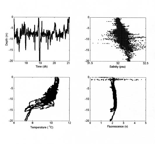
Figure 8.3. Data from the OS200 ctd mounted on the ROV during deployment ROV4 on the
Southern Flank. The ROV descended to a depth of 8 m oscillating vertically a few meters as it traveled forward
along the thermocline.
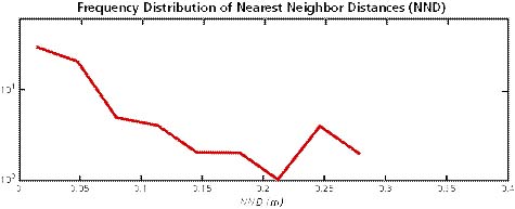

Figure 8.4. Log frequency distribution of the nearest neighbor distances (NND) between
adjacent Calanus sp. as the ROV traveled forward during ROV4 (TOP). Note two modes in the distribution:
scales less than ca 20 cm indicate NNDs within a patch, the second mode at scales greater than 25 cm indicate
a mean between patch distance.
Orientation of all Calanus sp. was divided almost equally between a head up and a head down
position (BOTTOM).
The linear decay at small scales on a semi log plot such as this indicates an exponential decrease in the frequency of NND as the dimensions increase. This is what would be expected if the organisms were randomly distributed within a volume. Thus the first mode of the distribution may indicate the distances between copepods within a given patch while the second mode indicates the mean distance between multiple patches. Table 8.1 provides some statistics on copepod patch structure for this short transect. Interestingly, copepod patches appeared on the order of 1 m in diameter and slightly less than a m3 in volume assuming spherical geometry. The interpatch distance was about 0.25 to 0.3 m. Mean copepod within patch density was 14,293 m-3 while the interpatch copepod density was four orders lower. The overall mean, integrated copepod concentration was about 2,200 m-3 suggesting a very patchy population. The smallest NNDs were on order 1 to 5 mm along with a few mating events being observed. Table 8.2 indicates that of those copepods within patches, none were swimming at detectable speeds. They were generally hanging motionless either directly upwards or directly downwards (Fig 8.4, bottom panel). The few copepods observed between patches were nearly all swimming either in loops or horizontally at an average speed of 0.046 m s-1 which for a 2 mm long adult Calanus indicates a relative speed of 23 body lengths per second. As suggested in the literature, this is typical of an escape velocity associated with escape from predation and defense. Nevertheless, as the ROV moved forward through patches, no copepods were observed to be disturbed by either the deep red light or any physical disturbance by the camera frame or ROV itself (i.e., the imaging system was not perceived as a threat). It may be, however, that what we have traditionally termed escapes are also used to rapidly locate patches of compatriots as the patch mass slowly diffuses outward. More data will need to be processed before we can conclude how patch structure changed with region or depth in the water column. Data on copepod swimming speed and direction as a function of depth and hydrographic conditions estimated from these analyses will then be incorporated into numerical models for determining transport of organisms along and across the front.
Table 8.1
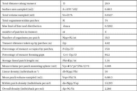
Table 8.2
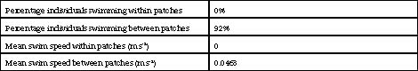
9. SHIPBOARD ADCP DATA ACQUISITION
Daniel J. Torres
The following describes the methods used to collect and process the shipboard ADCP data for GLOBEC legs EN323 AND EN324 aboard R/V Endeavor from May 6, 1999 to June 6, 1999. Shipboard ADCP data collected with a narrow band ADCP is typically collected on a 386 PC computer (herein referred to as the DAS computer) using RD Instruments DAS248 data acquisition software. One of the objectives for this cruise was to use the ADCP data to help track the spread of the dye patch as it evolved over time. In order to do this most effectively, absolute velocity from the ADCP was needed as close to real time as possible. So rather than ftp the data or worse yet, copy it to floppies, the data were written directly to an SGI file system exported to the DAS PC. The raw pingdata files were then run through a series of programs to produce .mat files of absolute velocity. These data were written to a directory which was being exported to a Linux PC which was doing the dye tracking. Absolute velocities were then integrated in time to track the spread of the dye patch. Outlined here are the steps for setting up all aspects of real time ADCP data acquisition and processing to absolute velocity.
A. DAS Setup
In order to maintain continuity with prior GLOBEC ADCP data, it was decided to use the Flagg setup for the ADCP DAS software. Based on geographic location and water depth, the Flagg autoadcp program determines which .cnf configuration file to use for the ADCP data acquisition. The changes involve adjustments to bin size and pulse length in order to maximize range and resolution in varying depths. Once autoadcp determines that a new .cnf file is required, the DAS PC automatically reboots with the new .cnf file in place. The only modifications needed for these files were to change the primary drive for writing the pingdata files from c: to d: and to change the secondary drive form d: to c: where drive d: is the SGI exported file system. The secondary drive is used if the primary drive is not available due to a crash or network interruption. These configuration files can be edited with any editor or from within the DAS program itself.
For the most part, the ADCP was configured to collect 50 bins of data every 4 meters. The center of the closest bin to the surface usually occurred at 11 meters depth. The sampling interval was 5 minutes for the whole cruise. Differential GPS was available throughout most of the cruise. Tansvector 3D GPS data were also collected in order to correct for the error in ship heading from the ship's gyro in postprocessing. However, in order to correct for the gyro error and transducer misalignment error during the cruise, a calibration method was developed to calculate the correction angle and apply it to the data in real time. This involved calculating the rms of absolute speed of a reference layer for different rotation angles. The final correction angle was found when the rms of speed converged to a minimum. The correction angle was then applied to the raw data as they were collected. Once the raw data were corrected for misalignment and gyro errors, absolute velocities were calculated. The final processed data were saved in daily Matlab mat files and exported to the Linux PC doing the dye tracking. Velocity vectors overlaid on bathymetry contours were also plotted in real time on the SGI.
B. DAS Network Connection
The DAS PC was initially set up on the Endeavor to collect data on its own c: drive. It was equipped with a network card but only had the drivers to connect it via ships network to a Windows NT machine. Since we were trying to connect to an SGI, a 3C509 combo card was used instead of the ship's NE2000 card. The 3C509 card pulled from another PC (WEBSTER) was well tested on WHOI's network. Using PCTCP software, the PC was configured on the science network. Here I differentiate science network from ship's network. Since ZIRCON (SGI used for data acquisition) and DYE (Linux PC used for dye tracking), were both part of the science network, it obviously made sense to put the DAS on the science network. To configure the DAS on the science network, all the pertinent network information was entered in c:\pctcp\pc_en323.ini file. This file contained IP addresses and other information required for network connection and mounting SGI file system on d: drive. The network and the mount was setup to occur automatically upon reboot. The autoexec.bat and config.sys were configured to do this. The PC runs DOS 6.2.11 and everything is done under DOS. No TSR's or other programs should be running to maximize available memory for network and for DAS to run properly.
C. SGI Network Connection
The SGI was configured on the science network in the usual way. A file system was exported from ZIRCON to DAS which was mounted by DAS as the d: drive. Due to a limitation in the DAS acquisition software, the file system exported by the SGI cannot be over 175 MB. Since I did not have an SGI disk that small, I found an old 1 Gig disk and repartitioned it to 2 file systems, one 750 MB and the other 150 MB. So my disks were partitioned as follows:
zircon 293% df
| Filesystem | Type | kbytes | use | avail | %use | Mounted on |
|---|---|---|---|---|---|---|
| /dev/root | xfs | 1962164 | 1342840 | 619324 | 69 | / |
| /dev/dsk/dks0d4s7 | xfs | 751244 | 88240 | 663004 | 12 | /zircon3 |
| /dev/dsk/dks0d4s6 | xfs | 150500 | 19564 | 130936 | 13 | /adcp |
| /dev/dsk/dks0d2s7 | efs | 4136080 | 3796487 | 339593 | 92 | /zircon2 |
The 150 MB partition /adcp was exported by adding the following line to /etc/exports file on ZIRCON: /adcp access=adcp.whoi.edu.
"adcp.whoi.edu" is the DAS computer. The default permissions were read/write so the DAS had access to write the data onto ZIRCON.
D. Processing Data
The processing of vmadcp data consists of converting raw ship relative velocities into absolute velocities. They involve the following steps in the order they are performed.
1. run_adcp_ship.m Matlab script which calls a series of programs that ultimately process the data into absolute velocity and plots it in various ways.
2. backadcp shell script for backing up pingdata files to a directory on another disk and catting together pingdata files into one big pingdata file.
3. rt_adcp1s.m Primary file for doing the actual calculations to convert ship relative velocity
into absolute velocity. This calls:
a. loadit_d.m: Matlab function which returns a series of Matlab variables and arrays
which contain the adcp raw data. Function loadit_d.m does this by calling:
b. bnl_p2m: C Program executable which reads the binary pingdata files. This is a version
of ping2mat from CODAS which has been modified by Flagg to read transducer temperature, bin
size, bin length, and bottom depth from the pingdata files. The data are read and saved as mat files.
c. find_misalign.m: Matlab function used for calculating transducer misalignment.
d. mat2xyz.m: Matlab program for saving processed absolute velocity data in daily mat files.
Once the data were processed, they were written to the DYE Linux PC and used for real-time dye tracking.
10. APPENDICES
Thermistors #1080 and 1085 and conductivity sensors #224 and 763 were the primary and secondary sensors used on the injection sled/CTD while thermistor 2266 and conductivity sensor 1804 were used on the VPR. The following table details the sensor calibrations. A salinity sample was taken by Niskin at 29 m depth during calibration cast 000 on May 15. Two samples were taken from the same Niskin and analyzed using a Guildline AutoSal 8400A. Both samples measured 32.6510 psu. Sensor #1804 read 32.6144, #224 read 32.6465, and #763 reported 32.6472 at 29 m on this cast.
| Sensor # | Calibration Date | Maximum Error (deg C) | Maximum Error (S/m) | Comments |
|---|---|---|---|---|
| 2266 | 15-Apr-99 | 0.00011 | VPR | |
| 2266 | 11-Dec-99 | 0.00088 | VPR | |
| 1804 | 15-Apr-99 | 0.00002 | VPR | |
| 1804 | 16-Dec-99 | 0.00180 | VPR | |
| 1080 | 10-Dec-98 | 0.00007 | Inject/CTD T0 | |
| 1080 | 16-Dec-99 | 0.00128 | Inject/CTD T0 | |
| 1085 | 10-Dec-98 | 0.00007 | Inject/CTD T1 | |
| 1085 | 16-Dec-99 | 0.00130 | Inject/CTD T1 | |
| 224 | 10-Dec-98 | 0.00008 | Inject/CTD C0 | |
| 224 | 21-Dec-99 | 0.00090 | Inject/CTD C0 | |
| 763 | 10-Dec-98 | 0.00004 | Inject/CTD C1 | |
| 763 | 21-Dec-99 | 0.00035 | Inject/CTD C1 |
On May 15, 1999 a test was performed to determine the difference, if any, between the sensors on the CTD sled used for injection of the dye, and the VPR sensors.
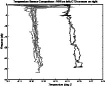
Figure10.1.1
Figure 10.1.1 shows the difference between the CTD temperature sensors and the VPR temperature sensor.
For data between 13 and 17 meters:
| T0 | T1 | VPR | |
|---|---|---|---|
| mean | 8.1554 | 8.1553 | 8.1233 |
| STD | .0014 | .0015 | .0015 |
| N | 331 | 331 | 303 |
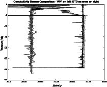
Figure 10.1.2
Figure 10.1.2 shows the difference between the CTD conductivity sensors and the VPR conductivity sensor. Note that computed Salinity is used to compare the data. The corresponding temperature sensor was used for the calculation (i.e. VPR Temperature sensor used for VPR salinity calculation)
For data between 13 and 17 meters:
| S0 | S1 | VPR | |
|---|---|---|---|
| mean | 32.6467 | 32.6475 | 32.6148 |
| STD | .000434 | .000407 | .000697 |
| N | 331 | 331 | 303 |
10.2 RHODAMINE FLUOROMETER CALIBRATIONS
The calibration method consists of filling a clean plastic barrel (#4 plastic, gray) with a 25-L aliquot of the receiving water for the tracer injection. It is important to use water as close as possible to the receiving waters since natural waters have varying trace constituents which might effect the background fluorescence. Calibrations with distilled, deionized water vary markedly from those in seawater for example. We have also seen background fluorescence change during a hydrocast in otherwise "clean" ocean water. Different layers of enhanced fluorescence, seemingly correlated to increased chlorophyll-a, suggest a biological origin. However, chlorophyll alone does not mean a higher rhodamine signal. In fact, usually the two fluorophors' signals are quite discrete. It is hypothesized that particular colonies of organisms, perhaps synecocochus bacteria, Cryptophyciae algae or their ilk containing phycoerytherin pigments, are fluorescing within the 580-600 nm emission wavelength sensed by the rhodamine fluorometer. Surface water (i.e. bucket samples) should also be avoided if possible because of the likelihood of surface films. Water can be acquired by pumping, if possible from the intended injection depth, with a submersible pump.
We have found that the calibration cell provided by Chelsea Instruments does not yield blank seawater voltage response values in concert with values seen when the instrument is deployed. Using the same batch of seawater, the Chelsea calibration cell showed a voltage of 1.46 while the same water in the 25-L plastic trash barrel provided only 1.15V. The latter value is very close to a representative average "blank" value observed in situ near the time and place of the calibration. The response using Chelsea's glass calibration cell appears likely dependent on handling and dilution technique, ambient lighting, and possibly background reflections or scattering from nearby objects. The Chelsea cell also inherently has air and glass interfaces that are not present when the whole unit is simply immersed in the ocean or standard solution. The larger measured dilution volumes and relative optical isolation inside the large dark bucket seem to minimize these problems. In addition, the calibration in the bucket is serial within one batch of water while the calibration cell requires as many separate dilutions as there are calibration points required, increasing the possibility of error. We were not able to reproduce Chelsea's quoted response in "reverse osmosis/ion exchange column" water using "Milli-Q" water. (Note: a standard blank water should have its resistivity specified for comparison)
Four dilutions and a blank were used in the calibration. First a secondary standard of 4.52E-5 g/g was made by diluting 100 µL of the 20% Intracid Rhodamine WT solution supplied by Crompton and Knowles in 500 mL of the receiving water. It should be noted that the same dye lot number should be used for the calibration as is intended for the tracer injection. Variations in Rhodamine WT lot concentration can be 2% as measured by the density of the 20% solution. In addition to the blank, secondary standard additions of 50 µL, 0.45 mL, 4.5 mL and 45 mL to the 25 L bucket yielded concentrations of 9E-11, 9E-10, 9E-9 and 9E-8 g/g respectively to cover nearly the full linear range of the Aquatracka. It is also important to record the temperature of the calibration water for later use since fluorescence is highly dependent on temperature. Observations of a standard solution have shown the following dependence of the sensitivity of the detector output on temperature:
VT= Vcal(1.027)T-Tcal
where Vcal is the voltage referenced to a calibration done at temperature Tcal for an observed voltage VT in water of temperature T. One additional observation worthy of note is that it appears that the output voltage drops slowly but significantly (approximately 0.01V/minute) as the solution sits in the bucket. Perhaps the dye is absorbed on the surfaces of the bucket. Hence, observations should be taken as soon as possible after thorough mixing of each standard addition has reasonably stabilized the output.
By combining the temperature correction and the overall calibration curve, tracer concentration is calculated using the following equation;
C = k (10VT - 10V0) / 1.027(T-Tcal)
where C is tracer concentration, k is the average point to point slope of concentration versus 10V (i.e. µC/µ10V) from the bucket dilutions, and V0 is the voltage in the zero addition water. K was found to be 0.010 for Aquatracka #162 and 0.0068 for #184. Tcal was 9°C for both instruments. We started with fluorometer 162 and switched to 184 at 1900 on 5/17 prior to VPR 12 and back to 162 at 1030 on 5/31 prior to VPR 29.
Science Party
| James R. Ledwell (Chief Scientist) | Woods Hole Oceanographic Institution |
| James H. Churchill (Scientist) | Woods Hole Oceanographic Institution |
| Carin J. Ashjian (Scientist) | Woods Hole Oceanographic Institution |
| Cabell S. Davis (Scientist) | Woods Hole Oceanographic Institution |
| Scott M. Gallager (Scientist) | Woods Hole Oceanographic Institution |
| Dennis McGillicuddy (Scientist) | Woods Hole Oceanographic Institution |
| Miles A. Sundermeyer (Scientist) | U. Mass/Dartmouth |
| Craig V. Lewis (Scientist) | Dartmouth College |
| Terence G. Donoghue (Technician) | Woods Hole Oceanographic Institution |
| Andrew P. Girard (Technician) | Woods Hole Oceanographic Institution |
| Cynthia J. Sellers (Technician) | Woods Hole Oceanographic Institution |
| Daniel J. Torres (Technician) | Woods Hole Oceanographic Institution |
| Valery Kosnyrev (Technician) | Woods Hole Oceanographic Institution |
| Qiao Hu (Technician) | Woods Hole Oceanographic Institution |
| Philip Alatalo (Technician) | Woods Hole Oceanographic Institution |
Ship's Personnel
| Rhett McMunn | Master |
| Bill Appleton | Chief Engineer |
| Elizabeth McCleod | Chief Mate |
| Dan Butler | Steward-1st leg |
| Dick Foley | Mate |
| Jack Buss | Boatswain |
| Bill Fanning | Marine Technician |
| Tom Hickey | Assistant Engineer |
| Tim Varney | Assistant Engineer |
| Glen Prouty | Able Bodied Seaman |
| Charlie Baker | Able Bodied Seaman |
| Craig Kerwick | Ordinary Seaman |
| Mike Butler | Messman-1st leg; Steward-2nd leg |
10.5 FILE LIST WITH SURVEY NUMBERS AND DESCRIPTIONS FOR USE WITH CRUISE TRACKS
Key to Table 10.5.1
VPR# The sequential number of the VPR lowering
SRVY # For compatibility with analysis software, this 'Survey Number' is used to designate data by Cruise, Experiment and Survey. This number is of the form c1sYZ; 'Y' is the experiment number. Experiment number '0' denotes single CTD casts rather than tow-yo surveys); 'Z' is the survey number (survey number '0' is denotes an injection). Experiment numbers are single digits (0-4) while survey number can exceed nine (9), e.g. c1s110 is experiment 1 survey 10
desc. This is a shorthand description of the survey
Time This is the GMT date and time of the beginning and end of each
hh mm survey in MM:DD:hh:mm format (MM - month; DD - day; hh - hour; mm - minute)
Table 10.5.1
| VPR # | SRVY # | desc. | Time St-End (GMT) mm:dd:hh:mm |
|---|---|---|---|
| EN323 | |||
| 2 | c1s00 | large scale survey | 05:06:23:52-05:08:00:32 |
| 3 | c1s01 | large scale survey | 05:08:06:48-05:09:08:21 |
| 5 | c1s02 | trim & test of AC9 | 05:09:12:41-05:09:17:16 |
| 6 | c1s03 | large grid | 05:09:20:59-05:10:19:57 |
| 7(ctd) | c1s04 | drifter recovery CTD's | 05:10:21:13-05:10:21:29 |
| 8(ctd) | 05:10:22:16-05:10:22:26 | ||
| 9(ctd) | 05:10:23:15-05:10:23:23 | ||
| 10(ctd) | 05:11:00:32-05:11:00:37 | ||
| 7 | c1s05 | 05:11:03:12-05:11:05:34 | |
| EN324 | |||
| 8 | c1s06 | pre-injection 1 large scale | 05:15:16:52-05:16:03:39 |
| 9 | lg sc | ||
| 10 | c1s07 | pre-injection 1 small scale | 05:16:08:58-05:16:16:53 |
| CTD 1,2 | c1s10 | Dye Release 1 | 05:16:17:22-05:16:18:31 |
| 11 | c1s11 | dye exp. 1 survey 1 | 05:16:18:55-05:16:22:15 |
| 11 | c1s12 | excursion to front and drifter deployment | 05:16:22:15-05:17:00:03 |
| 11 | c1s13 | dye exp. 1 survey 2 | 05:17:00:03-05:17:20:18 |
| (ROV ops) | |||
| 12 | c1s14 | dye exp. 1 survey 3 | 05:17:23:19-05:19:10:45 |
| 12 | c1s08 | excursion to slope | 05:19:10:45-05:19:15:48 |
| (pick up drifters) | |||
| (ROV trial) | |||
| 13 | c1s15 | large scale survey with some dye from exp. 1 | 05:20:04:53-05:21:08:48 |
| 13 | c1s16 | remainder of VPR #13 | 05:21:08:48-05:22:12:37 |
| 14/15 | c1s09 | pre-injection small scale survey near Houghton | 05:22:14:15-05:23:06:05 |
| 16 | c1s010 | pre-injection small scale survey in West | 05:23:07:35-05:23:14:30 |
| CTD 10 | c1s20 | Dye Release 2 | 05:23:17:41-05:23:18:28 |
| 17 | c1s21 | dye exp. 2 survey 1 (srvy 1) | 05:23:18:59-05:24:00:59 |
| 17 | c1s22 | excursion to front | 05:24:00:59-05:24:06:37 |
| (ROV ops) | |||
| 18 | c1s23 | 10x10km radiator survey | 05:24:08:36-05:25:00:28 |
| 18 | c1s24 | excursion to front | 05:25:00:28-05:25:04:32 |
| 18 | c1s25 | dye exp. 2 survey 2 | 05:25:04:32-05:25:18:29 |
| 18 | c1s26 | excursion to front | 05:25:18:29-05:25:22:19 |
| 18 | c1s27 | migration study | 05:25:19:12-05:27:00:25 |
| 19 | c1s28 | excursion to front | 05:27:00:39-05:27:03:49 |
| 20 | c1s011 | Biological front study | 05:27:06:52-05:27:09:39 |
| 20 | c1s012 | Front section | 05:27:09:39-05:27:13:56 |
| CTD 11 | c1s30 | Dye Release 3 | 05:27:18:26-05:27:18:46 |
| 21 | c1s31 | dye exp. 3 survey 1 | 05:27:15:05-05:27:16:51 |
| 22 | c1s29 | search for ROV location | 05:27:19:41-05:27:20:54 |
| 23 | c1s210 | dye exp. 2 survey 3 | 05:28:01:17-05:29:04:20 |
| 24 | c1s211 | excursion to front | 05:29:04:20-05:29:07:25 |
| 24 | c1s32 | dye exp. 3 survey 2 | 05:29:07:25-05:29:20:52 |
| 25 | |||
| 26 | c1s013 | initial large scale survey on North Flank | 05:30:03:06-05:31:03:06 |
| 27 | c1s014 | front section | 05:31:11:12-05:31:14:12 |
| 28 | |||
| 29 | c1s015 | pre-injection survey | 05:31:23:02-06:01:17:34 |
| CTD 15 | c1s40 | Dye Release 4 | 06:01:17:53-06:01:18:47 |
| 30 | c1s41 | dye exp. 4 survey 1 | 06:01:19:03-06:02:01:42 |
| c1s42 | dye exp. 4 survey 2 | 06:02:01:42-06:02:09:04 | |
| c1s43 | dye exp. 4 survey 3 | 06:02:09:04-06:02:15:35 | |
| c1s44 | dye exp. 4 survey 4 | 06:02:15:35-06:02:22:39 | |
| c1s45 | dye exp. 4 survey 5 | 06:02:22:39-06:03:10:06 | |
| c1s46 | dye exp. 4 survey 6 | 06:03:10:06-06:03:21:28 | |
| c1s47 | dye exp. 4 survey 7 | 06:03:21:28-06:04:22:37 | |
| c1s48 | dye exp. 4 survey 8 | 06:04:06:37-06:05:01:23 | |
| c1s49 | dye exp. 4 survey 9 | 06:05:01:57-06:06:08:14 |
Key to Table 10.5.2
This table key is similar to Table 10.5.1 but adds two columns, and shortens the description.
File: This is the name of the raw data file as provided by the VPR data logging scheme. The file name indicates MM:DD:hh:mm that the file was started. It is provided here for use by data analysts.
Time: This column represents the time in decimal year day (Jan 1 = day) and is provided since the time variable in the Matlab format files is represented in this way.
Desc: Abbreviated descriptions
Table 10.5.2
| VPR # | SRVY # | desc. | File |
Time St-End (GMT) decimal day | mm:dd:hh:mm |
|---|---|---|---|---|---|
| 2 | c1s00 | lg grd | 05062352_1 | 125.9948-126.2247 | 05:06:23:52-05:07:05:23 |
| 05062352_2 | 126.2247-126.4556 | 05:07:05:23-05:07:10:56 | |||
| 05062352_3 | 126.4556-126.6880 | 05:07:10:56-05:07:16:30 | |||
| 05062352_4 | 126.6881-126.9218 | 05:07:16:30-05:07:22:07 | |||
| 05062352_5 | 126.9218-127.0224 | 05:07:22:07-05:08:00:32 | |||
| 3 | c1s01 | lg grd | 05080648_1 | 127.2838-127.5138 | 05:08:06:48-05:08:12:19 |
| 05080648_2 | 127.5138-127.7447 | 05:08:12:19-05:08:17:52 | |||
| 05080648_3 | 127.7447-127.9757 | 05:08:17:52-05:08:23:24 | |||
| 05080648_4 | 127.9757-128.2089 | 05:08:23:24-05:09:05:00 | |||
| 05080648_5 | 128.2089-128.3484 | 05:09:05:00-05:09:08:21 | |||
| 5 | c1s02 | tst AC9 | 5091241 | 128.5290-128.7187 | 05:09:12:41-05:09:17:16 |
| 6 | c1s03 | lg grd | 5092059 | 128.8745-129.0531 | 05:09:20:59-05:10:01:16 |
| 05100116_1 | 129.0532-129.2845 | 05:10:01:16-05:10:06:49 | |||
| 05100116_2 | 129.2845-129.5158 | 05:10:06:49-05:10:12:22 | |||
| 05100116_3 | 129.5158-129.6035 | 05:10:12:22-05:10:14:29 | |||
| 5101516 | 129.6366-129.8314 | 05:10:15:16-05:10:19:57 | |||
| 7(ctd) | c1s04 | CTD | 5102113 | 129.8844-129.8956 | 05:10:21:13-05:10:21:29 |
| 8(ctd) | 5102216 | 129.9280-129.9348 | 05:10:22:16-05:10:22:26 | ||
| 9(ctd) | 5102315 | 129.9692-129.9743 | 05:10:23:15-05:10:23:23 | ||
| 10(ctd) | 5110032 | 130.0224-130.0264 | 05:11:00:32-05:11:00:37 | ||
| 7 | c1s05 | 5110312 | 130.1336-130.2325 | 05:11:03:12-05:11:05:34 | |
| 8 | c1s06 | pre inj1 | 5151651 | 134.7028-134.7801 | 05:15:16:52-05:15:18:43 |
| 9 | lg sc | 5152103 | 134.8777-134.9681 | 05:15:21:03-05:15:23:14 | |
| 05152314_1 | 134.9682-135.1526 | 05:15:23:14-05:16:03:39 | |||
| 10 | c1s07 | pre inj1 | 05160858_1 | 135.3741-135.6053 | 05:16:08:58-05:16:14:31 |
| sm sc | 05160858_2 | 135.6053-135.7037 | 05:16:14:31-05:16:16:53 | ||
| CTD 1,2 | c1s10 | Inj 1 | glob002a | 135.7236-135.7715 | 05:16:17:22-05:16:18:31 |
| 11 | c1s11 | dye 1 (srvy 1) | 05161855_1a | 135.2810-135.9272 | 05:16:18:55-05:16:22:15 |
| 11 | c1s12 | exc2frnt &dr depl | 05161855_1b | 135.9272-136.0025 | 05:16:22:15-05:17:00:03 |
| 11 | c1s13 | dye 1 | 05161855_1c | 136.0025-136.0217 | 05:17:00:03-05:17:00:31 |
| 05161855_2 | 136.0217-136.2578 | 05:17:00:31-05:17:06:11 | |||
| (srvy2) | 05161855_3 | 136.2578-136.4986 | 05:17:06:11-05:17:11:58 | ||
| 05161855_4 | 136.4987-136.7378 | 05:17:11:58-05:17:17:42 | |||
| 05161855_5 | 136.7378-136.8463 | 05:17:17:42-05:17:20:18 | |||
| (ROV ops) | |||||
| 12 | c1s14 | dye 1 | 5172319 | 136.9720-137.0040 | 05:17:23:19-05:18:00:05 |
| (srvy 3) | 5180005 | 137.0042-137.0241 | 05:18:00:05-05:18:00:34 | ||
| 5180038 | 137.0265-137.0287 | 05:18:00:38-05:18:00:41 | |||
| 05180058_1 | 137.0409-137.2720 | 05:18:00:58-05:18:06:31 | |||
| 05180058_2 | 137.2720-137.5049 | 05:18:06:31-05:18:12:07 | |||
| 05180058_3 | 137.5049-137.7388 | 05:18:12:07-05:18:17:43 | |||
| 05180058_4 | 137.7388-137.9738 | 05:18:17:43-05:18:23:22 | |||
| 05180058_5 | 137.9738-137.2103 | 05:18:23:22-05:19:05:02 | |||
| 05180058_6 | 137.2103-138.4480 | 05:19:05:02-05:19:10:45 | |||
| 12 | c1s08 | exc2slop | 05180058_7 | 138.4480-138.6584 | 05:19:10:45-05:19:15:48 |
| (pick up drifters) (ROV trial) | |||||
| 13 | c1s15 | ls svy | 05200453_1 | 139.2037-139.4360 | 05:20:04:53-05:20:10:27 |
| w/dye 1 | 05200453_2 | 139.4360-139.6719 | 05:20:10:27-05:20:16:07 | ||
| 05200453_3 | 139.6719-139.9080 | 05:20:16:07-05:20:21:47 | |||
| 05200453_4 | 139.9080-140.1456 | 05:20:21:47-05:21:03:29 | |||
| 05200453_5a | 140.1456-140.3668 | 05:21:03:29-05:21:08:48 | |||
| 13 | c1s16 | rest of | 05200453_5b | 140.3668-140.3822 | 05:21:08:48-05:21:09:10 |
| vpr 13 | 05200453_6 | 140.3823-140.5540 | 05:21:09:10-05:21:13:17 | ||
| 05211318_1 | 140.5542-140.7895 | 05:21:13:18-05:21:18:56 | |||
| 05211318_2 | 140.7895-141.0246 | 05:21:18:56-05:22:00:35 | |||
| 05211318_3 | 141.0246-141.2605 | 05:22:00:35-05:22:06:15 | |||
| 05211318_4 | 141.2606-141.3580 | 05:22:06:15-05:22:08:35 | |||
| 05220859_1 | 141.3749-141.5261 | 05:22:08:59-05:22:12:37 | |||
| 14/15 | c1s09 | pre inj | 05221415_1 | 141.5939-141.7951 | 05:22:14:15-05:22:19:04 |
| sm sc nr | 05221941_1 | 141.8204-142.0567 | 05:22:19:41-05:23:01:21 | ||
| Houghton | 05221941_2 | 142.0567-142.2538 | 05:23:01:21-05:23:06:05 | ||
| 16 | c1s010 | pre inj | 05230735_1 | 142.3163-142.5559 | 05:23:07:35-05:23:13:20 |
| sm sc in West | 05230735_2 | 142.5559-142.6044 | 05:23:13:20-05:23:14:30 | ||
| CTD 10 | cls20 | inj 2 | glob010a,b | 142.7368-142.7694 | 05:23:17:41-05:23:18:28 |
| 17 | c1s21 | dye 2 | 05231859_1 | 142.7916-143.0330 | 05:23:18:59-05:24:00:47 |
| (srvy 1) | 05231859_2a | 143.0330-143.0417 | 05:24:00:47-05:24:00:59 | ||
| 17 | c1s22 | exc2frnt | 05231859_2b | 143.0417-143.2749 | 05:24:00:59-05:24:06:35 |
| 05231859_3 | 143.2749-143.2758 | 05:24:06:35-05:24:06:37 | |||
| (ROV) | |||||
| 18 | c1s23 | 10x10km | 05240836_1 | 143.3584-143.6014 | 05:24:08:36-05:24:14:26 |
| radiator | 05240836_2 | 143.6015-143.8428 | 05:24:14:26-05:24:20:13 | ||
| 05240836_3a | 143.8428-144.0200 | 05:24:20:13-05:25:00:28 | |||
| 18 | c1s24 | exc2frnt | 05240836_3b | 144.0200-144.0859 | 05:25:00:28-05:25:02:03 |
| 05240836_4 | 144.0859-144.1892 | 05:25:02:03-05:25:04:32 | |||
| 18 | c1s25 | dye 2 | 05250432_1 | 144.1893-144.3143 | 05:25:04:32-05:25:07:32 |
| (srvy 2) | 05250432_2 | 144.3143-144.4375 | 05:25:07:32-05:25:10:30 | ||
| 05250432_3 | 144.4376-144.5607 | 05:25:10:30-05:25:13:27 | |||
| 05250432_4 | 144.5607-144.6810 | 05:25:13:27-05:25:16:20 | |||
| 05250432_5a | 144.6810-144.7708 | 05:25:16:20-05:25:18:29 | |||
| 18 | c1s26 | exc2frnt | 05250432_5b | 144.7708-144.8005 | 05:25:18:29-05:25:19:12 |
| 05251912_1a | 144.8006-144.9304 | 05:25:19:12-05:25:22:19 | |||
| 18 | c1s27 | migrat. | 05251912_1 | 144.8006-145.0366 | 05:25:19:12-05:26:00:52 |
| stdy | 05251912_2 | 145.0366-145.2769 | 05:26:00:52-05:26:06:38 | ||
| 05251912_3 | 145.2769-145.5164 | 05:26:06:38-05:26:12:23 | |||
| 05251912_4 | 145.5164-145.7592 | 05:26:12:23-05:26:18:13 | |||
| 05251912_5 | 145.7592-145.9980 | 05:26:18:13-05:26:23:57 | |||
| 05251912_6 | 145.9980-146.0180 | 05:26:23:57-05:27:00:25 | |||
| 19 | c1s28 | exc2frnt | 05270039_1 | 146.0277-146.1448 | 05:27:00:39-05:27:03:28 |
| 05270039_2 | 146.1448-146.1594 | 05:27:03:28-05:27:03:49 | |||
| 20 | c1s011 | Bio. Ft stdy | 05270652_1a | 146.2864-146.4023 | 05:27:06:52-05:27:09:39 |
| 20 | c1s012 | Front | 05270652_1b | 146.4023-146.4520 | 05:27:09:39-05:27:10:50 |
| sec. | 05271051_1 | 146.4521-146.4796 | 05:27:10:51-05:27:11:30 | ||
| 05271130_1 | 146.4798-146.5809 | 05:27:11:30-05:27:13:56 | |||
| c1s30 | inject 3 | glob011a | 146.7681-146.7799 | 05:27:18:26-05:27:18:46 | |
| 21 | c1s31 (srvy 1) | dye 3 | 05271505_1 | 146.6286-146.7026 | 05:27:15:05-05:27:16:51 |
| 22 | c1s29 | sch for ROV loc | 05271941_1 | 146.8208-146.8711 | 05:27:19:41-05:27:20:54 |
| 23 | c1s210 | dye 2 | 05280117_1 | 147.0536-147.2887 | 05:28:01:17-05:28:06:55 |
| (srvy 3) | 05280117_2 | 147.2162-147.5258 | 05:28:06:55-05:28:12:37 | ||
| 05280117_3 | 147.5258-147.7635 | 05:28:12:37-05:28:18:19 | |||
| 05280117_4 | 147.7635-147.8998 | 05:28:18:19-05:28:21:35 | |||
| 05290037_1 | 148.0258-148.0354 | 05:29:00:37-05:29:00:51 | |||
| 05290051_1a | 148.0356-148.1812 | 05:29:00:51-05:29:04:20 | |||
| 24 | c1s211 | front | 05290051_1b | 148.1812-148.2713 | 05:29:04:20-05:29:06:30 |
| section | 05290051_2a | 148.2713-148.3094 | 05:29:06:30-05:29:07:25 | ||
| 24 | c1s32 | dye 3 | 05290051_2b | 148.3094-148.5088 | 05:29:07:25-05:29:12:12 |
| (srvy) | (srvy 2) | 05290051_3 | 148.5088-148.7007 | 05:29:12:12-05:29:16:48 | |
| 25 | 05291721_1 | 148.7233-148.8695 | 05:29:17:21-05:29:20:52 | ||
| 26 | c1s013 | initial | 05300306_1 | 149.1294-149.3664 | 05:30:03:06-05:30:08:47 |
| srvy N. | 05300306_2 | 149.3664-149.6059 | 05:30:08:47-05:30:14:32 | ||
| 05300306_3 | 149.6059-149.8474 | 05:30:14:32-05:30:20:20 | |||
| 05300306_4 | 149.8474-150.0904 | 05:30:20:20-05:31:02:10 | |||
| 05300306_5 | 150.0904-150.1292 | 05:31:02:10-05:31:03:06 | |||
| 27 | c1s014 | front | 05311112_1 | 150.4672-150.4750 | 05:31:11:12-05:31:11:23 |
| 28 | section | 05311317_1 | 150.5542-150.5923 | 05:31:13:17-05:31:14:12 | |
| 29 | c1s015 | pre-inj | 05312302_1 | 150.9604-151.1968 | 05:31:23:02-06:01:04:43 |
| 05312302_2 | 151.1968-151.4395 | 06:01:04:43-06:01:10:32 | |||
| 05312302_3 | 151.4395-151.5345 | 06:01:10:32-06:01:12:49 | |||
| 06011249_1 | 151.5346-151.7322 | 06:01:12:49-06:01:17:34 | |||
| c1s40 | inject 4 | glob015a | 151.7451-151.7826 | 06:01:17:53-06:01:18:47 | |
| 30 | c1s41 | dye 4 | 06011903_1a | 151.7942-152.0301 | 06:01:19:03-06:02:00:43 |
| (srvy 1) | 06011903_2a | 152.0301-152.0712 | 06:02:00:43-06:02:01:42 | ||
| c1s42 | dye 4 | 06011903_2b | 152.0712-152.2685 | 06:02:01:42-06:02:06:26 | |
| (srvy 2) | 06011903_3a | 152.2685-152.3781 | 06:02:06:26-06:02:09:04 | ||
| c1s43 | dye 4 | 06011903_3b | 152.3781-152.5097 | 06:02:09:04-06:02:12:13 | |
| (srvy 3) | 06011903_4a | 152.5097-152.6498 | 06:02:12:13-06:02:15:35 | ||
| c1s44 | dye 4 | 06011903_4b | 152.6498-152.7526 | 06:02:15:35-06:02:18:03 | |
| (srvy 4) | 06011903_5a | 152.7526-152.9439 | 06:02:18:03-06:02:22:39 | ||
| c1s45 | dye 4 | 06011903_5b | 152.9439-152.9906 | 06:02:22:39-06:02:23:46 | |
| (srvy 5) | 06011903_6a | 152.9906-153.2447 | 06:02:23:46-06:03:05:52 | ||
| 06011903_7a | 153.2447-153.4209 | 06:03:05:52-06:03:10:06 | |||
| c1s46 | dye 4 | 06011903_7b | 153.4209-153.5058 | 06:03:10:06-06:03:12:08 | |
| (srvy 6) | 06011903_8a | 153.5058-153.5120 | 06:03:12:08-06:03:12:17 | ||
| 06031259_1a | 153.5414-153.7813 | 06:03:12:59-06:03:18:45 | |||
| 06031259_2a | 153.7813-153.8951 | 06:03:18:45-06:03:21:28 | |||
| c1s47 | dye 4 | 06031259_2b | 153.8951-154.0192 | 06:03:21:28-06:04:00:27 | |
| (srvy 7) | 06031259_3a | 154.0192-154.2584 | 06:04:00:27-06:04:06:12 | ||
| 06031259_4a | 154.2584-154.9424 | 06:04:06:12-06:04:22:37 | |||
| c1s48 | dye 4 | 06031259_4b | 154.2757-154.4969 | 06:04:06:37-06:04:11:55 | |
| (srvy 8) | 06031259_5a | 154.4969-154.7416 | 06:04:11:55-06:04:17:47 | ||
| 06031259_6a | 154.7416-154.8452 | 06:04:17:47-06:04:20:17 | |||
| 06042017_1a | 154.8455-155.0577 | 06:04:20:17-06:05:01:23 | |||
| c1s49 | dye 4 | 06050157_1 | 155.0815-155.3215 | 06:05:01:57-06:05:07:42 | |
| (srvy 9) | 06050157_2 | 155.3215-155.5608 | 06:05:07:42-06:05:13:27 | ||
| 06050157_3 | 155.5608-155.7734 | 06:05:13:27-06:05:18:33 | |||
| 06052322_1 | 155.9738-156.2176 | 06:05:23:22-06:06:05:13 | |||
| 06052322_2 | 156.2176-156.3435 | 06:06:05:13-06:06:08:14 |
The upper panel shows location of the centers of the tow-yo profiles in original coodinates. The lower panel shows the location advected to a common time by integrating the ADCP data at the ship. The Schlitz moorings are shown as open circles. The start of each survey is indicated with a circle around a dot. The end with an 'x.' Each dot along the track indicates a tow-yo profile, either up or down. An isobath, usually the 60-m isobath, is shown to help locate each survey relative to the Bank and to the tidal mixing front. The tracks are all labelled as "surveys," although this is not always an appropriate name.
Please note: Some of these images did not transfer very well to the web. See the written cruise report for the true track plots. (DMO)