HYDROGRAPHIC SURVEY REPORT
Technical Report UNH-OPAL-1998-005
Convective Overturn Experiment
(CONVEX) CRUISE # 6
R/V OCEANUS (OC-316)
(Between 29 January and 02 February 1998)
F. L. Bub, W. S. Brown, & L. C. Smith
Ocean Process Analysis Laboratory (OPAL)
Institute for the Study of Earth, Ocean and Space
Department of Earth Sciences
University of New Hampshire
Durham, NH 03824
Research Sponsored by the National Science Foundation
Report Contents.
0. Abstract
1. Introduction
2. Cruise Narrative
3. Data
3a. Data Acquisition
3b. Processing
3c. Corrections
3d. Presentations
4. Acknowledgements
5. References
Tables.
Table 1. Surface Contours of Properties on Pressure and Density Surfaces.
Table 2. CTD Station Information.
Figures.
Figure 1.a. Cruise Track, CTD Locations and UNH mooring sites. Stations
numbered sequentially.
Figure 1.b. Station and mooring locations with Wilkinson Basin bathymetry and
water mass analysis region outlined.
Figure 2. Wilkinson Basin mooring configuration showing the Main Buoy (A),
thermistor chains (B & C), and guard buoys (D, E & G).
Figure 3.a.. Composite of CTD profiles in Wilkinson Basin. See
section 3.d.1 for a description.
Figure 3.b.. Temperature-Salinity Diagram for CTD profiles in
Wilkinson Basin.
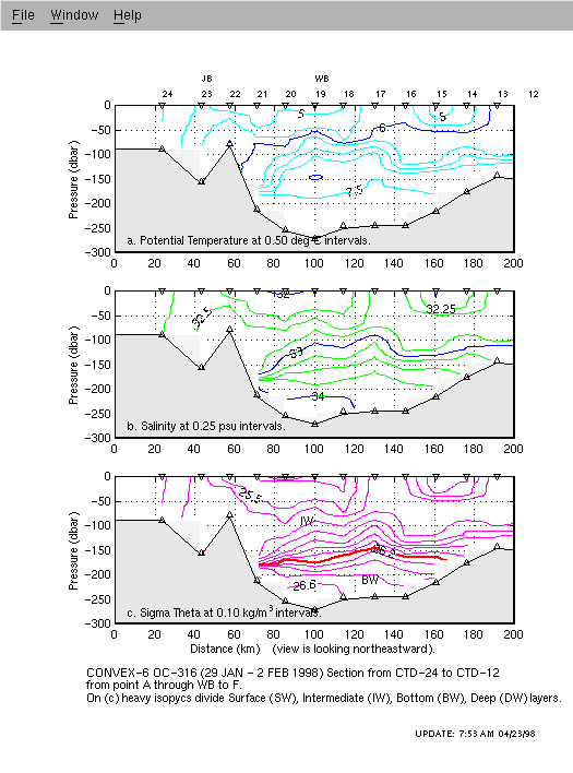
Figure 4.a. Hydrography Section A to F: Stations 24-12. Vertical
sections of temperature / salinity / sigma theta.
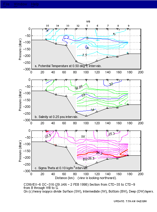
Figure 4.b. Hydrography Section B to G: Stations 35-32, 05-09.
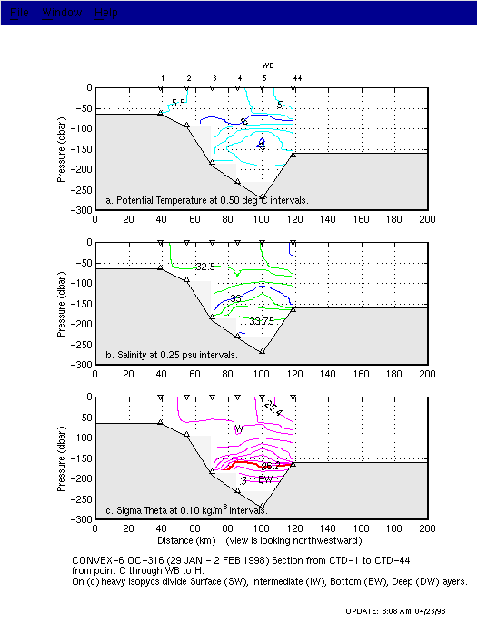
Figure 4.c. Hydrography Section C to H: Stations 01-05, 44.
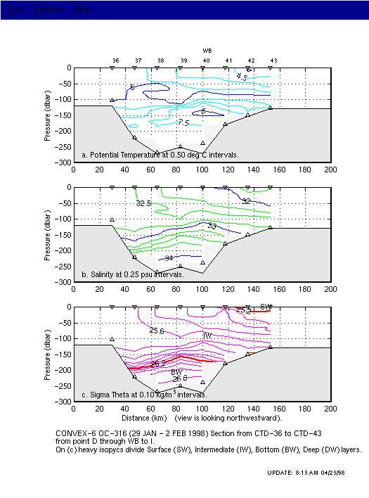
Figure 4.d. Hydrography Section D to I: Stations 36-43.
Figure 4.e. Hydrography Section J to E: Stations 26-31, 45-47, 49.
Figure 4.f. Hydrography Section C to F,G: Stations 01, 38, 46, 15, 10.
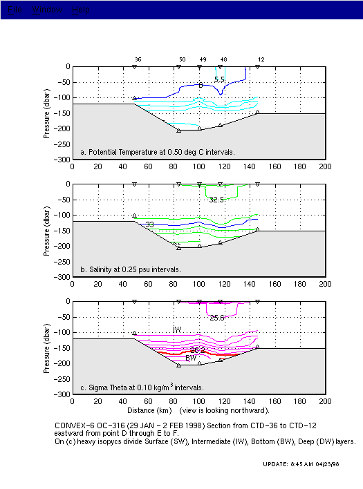
Figure 4.g. Hydrography Section D to F: Stations 36, 50, 49, 48, 12.
This report describes a set of hydrographic measurements obtained 29 January - 02 February 1998 as part of
the NSF-supported "Observational / Modeling Study of Wintertime Convection and Water Mass Formation"
in the western Gulf of Maine (GOM). Herein we document the sixth of seven planned University of New
Hampshire (UNH) cruises aboard the R/Vs ENDEAVOR and OCEANUS as part of this "Convective Overturn
Experiment" (CONVEX). This report and these data can be accessed through the RMRP Research Environmental
Data and Information Management System (REDIMS) via the WWW address:
http://ekman.sr.unh.edu/OPAL/CONVEX/
Click here to read an introduction to the CONVEX program.
After a two hour delay to allow high winds to abate, the RV OCEANUS departed Woods Hole at 1100L (1600Z)
on 29 January 1998. After a transit via Cape Cod Canal, we arrived at the first hydrographic station
at the start of transect "C" at 2000L. With the exception of time spent checking central Wilkinson Basin
mooring functions and determining precise locations on 30 January, entire cruise dedicated to hydrographic
survey.
A total of 50 CTD profiles were collected (Figure 1.a.),
along with 7 "bongo net" plankton tows for A. Bucklin. We also deployed a drifter for R. Limeburner.
The last profile was completed 0110L 2 February and the ship returned to WHOI via Nantucket Shoals,
docking approximately 0830 on 2 Feburary 1998.
2.a. Scientific Party.
F. L. Bub (Chief Scientist), W. S. Brown, K. Garrison, P. Mupparapu, B. Strully, J. Salisbury, J. Lund,
J. R. Rogers, N. Mottola, L Smith.
2.b. Cruise Photos.
Click here to see CONVEX Cruise photos. Miscellaneous
CONVEX GIF photos are included.
The R/V OCEANUS' SeaBird SBE 911 Plus CTD Profiler was used to measure
vertical profiles of electrical conductivity and temperature versus pressure at 50 hydrographic stations during
29 January - 2 February 1998 (Figure 1.a).
Sensors on the CTD were factory calibrated on 9 October 1996. This CTD samples at a rate of 24 scans per second.
Salinity profiles were computed from these data using SeaBird software. Additional
sensors on the SBE-911 also recorded data for the measurement of dissolved oxygen, water transmissivity, fluorescence
(Chl-a), and irradiance (PAR). Data acquisition, display and storage were managed by an on-board computer using the
SeaBird software package SEASOFT.
At each station, the CTD was lowered at a rate of approximately 30 meters per minute to depths within 5-10 meters of
the bottom. Three to eight water samples were collected with a rossette of 5-liter Niskin bottles, and specimens for
nutrient and oxygen isotope analyses were gathered. For each station, the condutivity of one water sample was determined
using the UNH Guildline 8400A Autosal and the corresponding salinities were used to correct salinity values derived from
the raw CTD measurements.
The CTD data were processed using a series of SeaBird SEASOFT programs (listed in parentheses) in which:
- a. Raw hexidecimal CTD output is converted into engineering units (DATCNV). Only downcast data were used
to produce station profiles. Bottles samples were taken during upcasts and average CTD data at each bottle depth
were stored (ROSSUM).
- b. Noise contamination greater than 2 standard deviations from 50 point sections was removed (WILDEDIT).
In addition, CTD downcast data associated with downward velocities of less than 25 cm/s (due to looping) were
discarded (LOOPEDIT).
- c. Data were filtered to ensure consistent response times using a low pass filter with time constant 0.15
sec (FILTER).
- d. Data were averaged into 1 decibar (dbar) bins (BINAVG) to produce profiles of temperature, salinity, etc.,
versus pressure from the unequally-spaced cast data from each station.
- e. These profile data were stored as ASCII files on floppy disks for post-processing and plotting.
Click here for a summary of data descriptions, corrections and estimated accuracy
/ precision.
The corrected hydrographic data are presented as:
- Station profile plots and property-property diagrams,
- Vertical section contour plots, and
- Horizontal pressure and desnity surface contour plots.
3.d.1. Vertical CTD Profile Plots.
Individual profiles may be viewed via Table 2. A composite of all CTD profiles
is shown as Figure 3.a and an expanded T-S diagram as
Figure 3.b. Data are presented on two pages per station:
- Page A - Station profiles of temperature, salinity, sigma-theta density, stability (N-squared) and a
temperature-salinity diagram. The upper three plots (surface to 100 m deep) represent zoomed details of water property
structure in the main thermocline (halocline, pycnocline) zone (horizontal scales vary). The middle plots present
these water property structures for the entire water column. These plots are all on the same depth / property
scale for intercomparison. A Brunt-Vaisaila frequency (N-squared) plot indicates water column stability.
- Page B - When data are available, this page shows station profiles of measured dissolved oxygen,
transmissivity, fluorescence (Chl-a), solar irradiance (PAR), as well as computed sound velocity, temperature -
dissolved oxygen, and salinity - dissolved oxygen diagrams.
3.d.2. Vertical Hydrographic Sections.
Potential temperature, salinity, and sigma-theta sections for the following transects are presented.
Each plot spans 200 km and horizontal scales are preserved. Contour intervals are indicated on plots.
The CTD station numbers are shown along the top horizontal axis and the ocean bottom (based on depths
at CTD stations) is shaded.
- Point A to F, tracking southeastward through Jeffreys and Wilkinson Basins
(Figure 4.a).
- Point B to G, tracking eastward through Massachusetts Bay and Wilkinson Basin
(Figure 4.b).
- Point C to H, tracking northeastward through Wilkinson Basin (Figure 4.c).
- Point D to I, tracking northeastward through Wilkinson Basin (Figure 4.d).
- Point J to E, tracking southward across Wilkinson Basin (Figure 4.e).
- Point C to F/G, tracking eastward across the southern Wilkinson Basin (Figure 4.f).
- Point D to F, tracking eastward across the southern Wilkinson Basin (Figure 4.g).
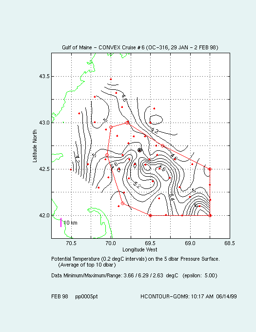
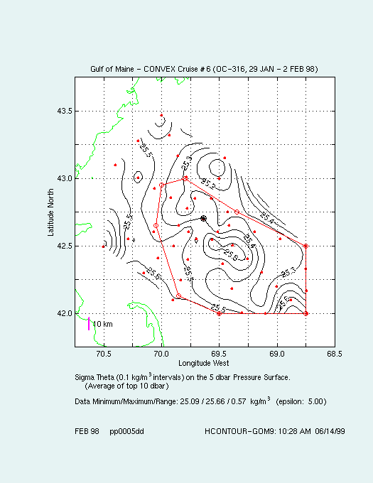
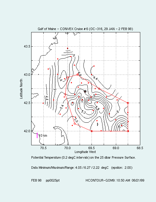
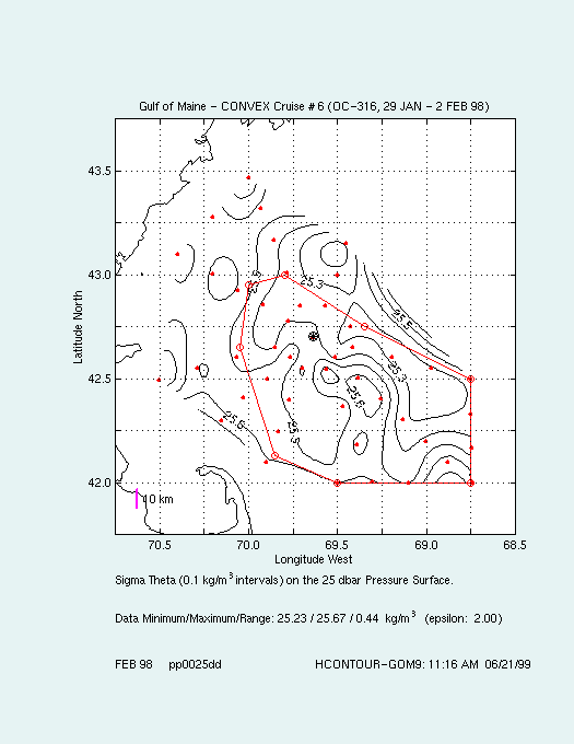
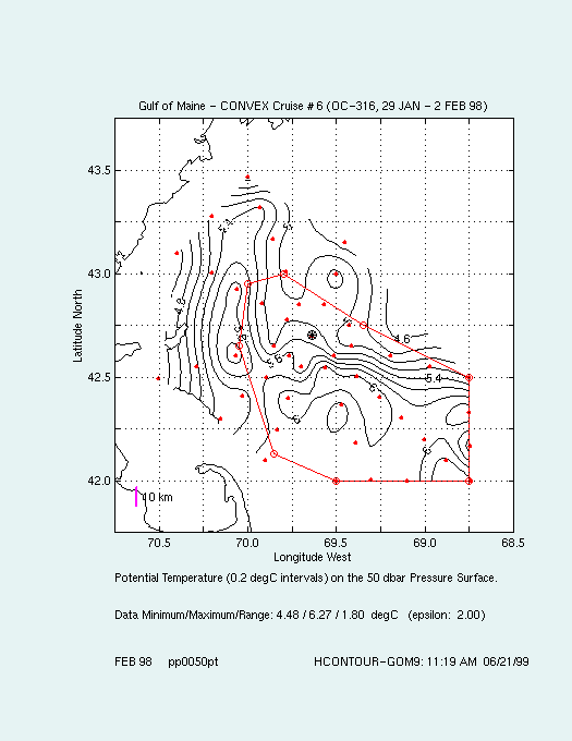
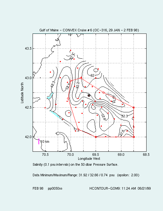
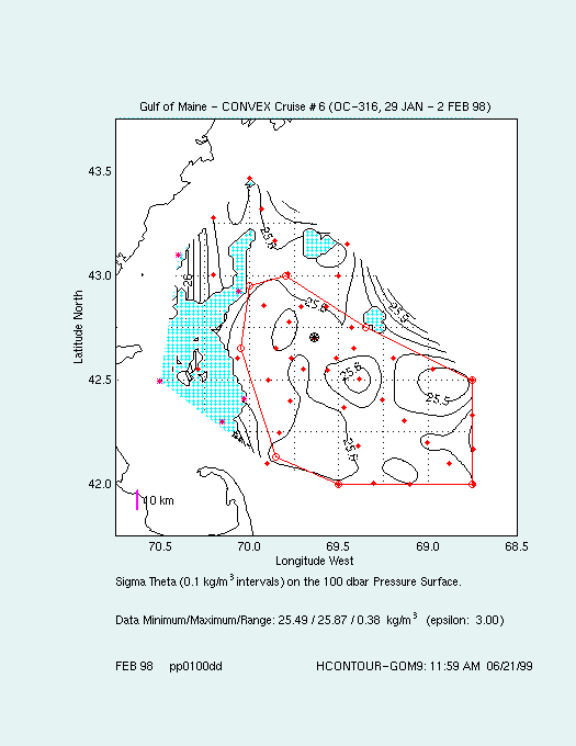
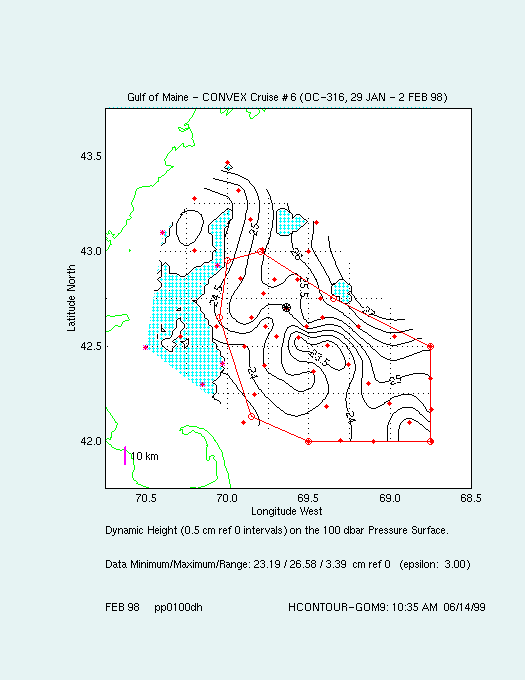
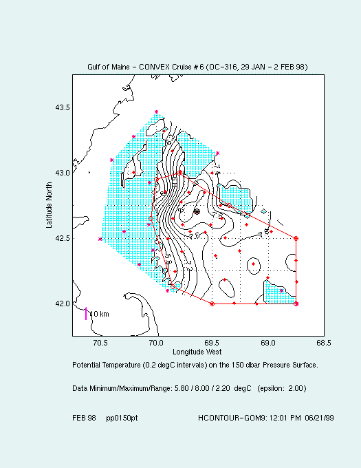
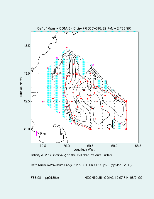
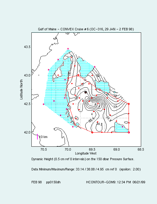
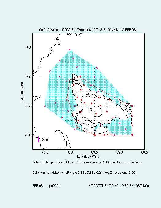
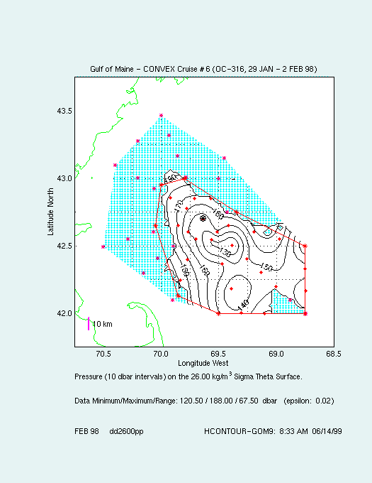
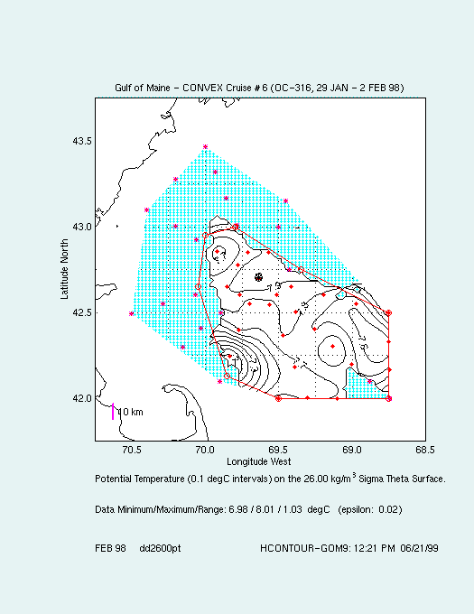
3.d.3. Horizontal Pressure and Density Surfaces.
Contoured surfaces may be accessed via Table 1.
Contours of temperature, salinity and density fields on the 5, 25, 50, 100, 150 and 200 dbar pressure surfaces
(equivalent to depth in m) and the sigma theta 26.00 density surface (mid water column) are presented for information.
The 5 m field is the mean of the 0-10 m layer. Dynamic height fields indicate geostrophic shear.
Cyan regions show where the ocean bottom is shallower than the plotted surface.
CTD profiles at the red dots (x indicates no data). Wilkinson Basin mooring marked by the wheel.
Red lines bound region of the CONVEX water mass analyses. Plotted contour intervals, along with data extrema and
search epsilon, are indicated in captions.
3.d.4. Data Files.
Profiles can be made available as (a) ASCII files upon request to
frank.bub@unh.edu.
Upon final quality control, we will provide (b) JGOFS default files through a ftp site.
Other OC-316 Cruise data including enroute ADCP, TSAL, navigation, bathymetry and observed weather records
will also be made available upon further processing.
We appreciate the efforts of Captain Bearse and the crew of R/V OCEANUSably as they preofessionally helped us conduct
this field program. The technical assistance of L. Stein is appreciated. We are grateful for the help provided by
T. Loder and R. Clauss in processing the bottle salinities. F. Bub, W. Brown, and P. Mupparapu are supported by NSF
Grant OCE-9530249.
Fofonoff, N. P. and R. C. Millard Jr., 1983. Algorithms for compilation of fundamental properties of seawater,
UNESCO Technical Papers in Marine Science, no. 44. UNESCO, Paris, France, 53 pages.
Garrison, K. M. and W. S. Brown, 1989. Hydrographic survey in the Gulf of Maine July-August 1987, UNH Tech.
Rpt. No. UNHMP-T/DR-SG-89-5, Univ. of NH, Durham, NH.
Morgan, P. P., 1994, SEAWATER Software Version 1.2b, CSIRO Division of Oceanography, Hobart, AUS.
These fields are briefly described in section 3.d.3. Pressure (P),
Temperature (T), Salinity (S), Density (D), and Dynamic Height (DH) are contoured at the specfied
pressure or density levels.
DENSITY
SURFACE
(kg/m^3) |
PRESSURE
(dbar) |
POTENTIAL
TEMPERATURE
(deg C) |
SALINITY
(psu) |
| 26.00 sigma theta |
P26.00 |
T26.00 |
S26.00 |
Hydrographic station information for the R/V OCEANUS Cruise OC-316 (29 January-02 February 1998). Position,
depth, date, and time are for the bottom of the cast. Profiles, which are described in
section 3.d.1, may be viewed by clicking on ##A or ##B. See Figure 1.a
for station locations.
 CTD station    Latitude    Longitude   Water Depth  Time     Date
   number      (deg min N)  (deg min W)  (meters)    (Z)   (DD/MM/YY)
________________________________________________________________________

01a   01b       42.2985      70.1532       64       0059   30/01/98
02a   02b       42.4058      70.0305       95       0204   30/01/98
03a   03b       42.4998      69.8958      190       0347   30/01/98
04a   04b       42.6000      69.7685      233       0514   30/01/98
05a   05b       42.6967      69.6422      270       0643   30/01/98
06a   06b       42.6490      69.4140      240       0824   30/01/98
07a   07b       42.6002      69.1928      210       0957   30/01/98
08a   08b       42.5492      68.9762      205       1126   30/01/98
09a   09b       42.4993      68.7508      185       1256   30/01/98
10a   10b       42.3287      68.7500      180       1418   30/01/98
11a   11b       42.1655      68.7472      200       1626   30/01/98
12a   12b       41.9972      68.7485      150       1745   30/01/98
13a   13b       42.0962      68.8798      146       1907   30/01/98
14a   14b       42.1997      69.0058      175       2013   30/01/98
15a   15b       42.3017      69.1310      216       2123   30/01/98
16a   16b       42.4035      69.2558      245       2238   30/01/98
17a   17b       42.5025      69.3858      245       2343   30/01/98
18a   18b       42.6040      69.5137      250       0046   31/01/98
19a   19b       42.6982      69.6360      270       0243   31/01/98
20a   20b       42.7773      69.7810      255       0351   31/01/98
21a   21b       42.8530      69.9198      215       0543   31/01/98
22a   22b       42.9258      70.0605       83       0649   31/01/98
23a   23b       43.0010      70.2003      160       0751   31/01/98
24a   24b       43.0975      70.4022       89       0909   31/01/98
25a   25b       43.2788      70.2003      102       1045   31/01/98
26a   26b       43.4682      70.0028      106       1225   31/01/98
27a   27b       43.3163      69.9302      152       1404   31/01/98
28a   28b       43.1633      69.8587      180       1512   31/01/98
29a   29b       43.0075      69.7857      177       1621   31/01/98
30a   30b       42.8525      69.7120      200       1734   31/01/98
31a   31b       42.6980      69.6367      270       1858   31/01/98
32a   32b       42.6488      69.8548      244       2246   31/01/98
33a   33b       42.6007      70.0698      125       2358   31/01/98
34a   34b       42.5502      70.2863      110       0107   01/02/98
35a   35b       42.4947      70.5018       83       0210   01/02/98
36a   36b       42.0968      69.9038      120       0712   01/02/98
37a   37b       42.2467      69.8352      225       0839   01/02/98
38a   38b       42.3978      69.7695      270       1017   01/02/98
39a   39b       42.5522      69.7012      252       1144   01/02/98
40a   40b       42.7008      69.6383      270       1255   01/02/98
41a   41b       42.8518      69.5712      180       1530   01/02/98
42a   42b       43.0000      69.5002      153       1638   01/02/98
43a   43b       43.1518      69.4527      128       1803   01/02/98
44a   44b       42.7483      69.4257      160       2034   01/02/98
45a   45b       42.5467      69.5613      285       2209   01/02/98
46a   46b       42.3633      69.4735      230       2328   01/02/98
47a   47b       42.1822      69.3893      195       0144   02/02/98
48a   48b       41.9995      69.1027      190       0335   02/02/98
49a   49b       42.0018      69.3030      205       0443   02/02/98
50a   50b       41.9995      69.5047      205       0606   02/02/98