 Figure 1. Standard station (large dots with numbers)
and intermediate stations (small dots) sampled along the
trackline traversed on OCEANUS cruise 319.
Figure 1. Standard station (large dots with numbers)
and intermediate stations (small dots) sampled along the
trackline traversed on OCEANUS cruise 319.ACKNOWLEDGEMENTS
We thank the captain and crew of the R/V OCEANUS for an enjoyable and productive cruise; their professionalism was greatly appreciated. In spite of high winds and rough seas on a portion of the cruise, most of the work was accomplished with extremely good results.
This report was prepared by Peter Wiebe, David Mountain, John Sibunka, Maria Casas, David Townsend, Jennifer Crain, and Rebecca Jones with assistance from others in the Scientific Party. This cruise was sponsored by the National Science Foundation and the National Oceanographic and Atmospheric Administration.
TABLE OF CONTENTS
Zooplankton and Ichthyoplankton studies based on Bongo and MOCNESS tows.
Preliminary Summary of Zooplankton Findings.
Samples Collected by the Zooplankton and Ichthyoplankton Groups:
Preliminary Summary of Ichthyoplankton Findings
Cod (Gadus morhua) and/or Pollock (Pollachius virens)
Haddock (Melanogrammus aeglefinnus)
Preliminary Summary of the 10-m2 MOCNESS samples.
Prey Size, Abundance and Motility Experiments Purpose
Phytoplankton chlorophyll, nutrients and light attenuation studies.
Greene Bomber Recovery In a Gale
Along track Environmental and ship MET Sensor Data
Shipboard ADCP (Acoustic Doppler Current Profiler) measurements.
APPENDIX 1. Event Log for R/V OCEANUS Cruise 319.
APPENDIX 2. Summary of observation made on zooplankton and ichthyoplankton.
Zooplankton observations made from 1-m2 MOCNESS net #0
Ichthyoplankton and zooplankton observations of the 10-m2 MOCNESS.
APPENDIX 3. CTD plots and compressed listing of the data.
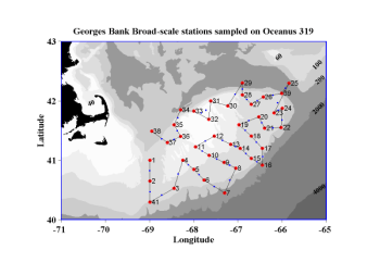
Figure 1. Standard station (large dots with numbers)
and intermediate stations (small dots) sampled along the
trackline traversed on OCEANUS cruise 319.The U.S. GLOBEC Georges Bank Program is now into its fourth full field season and this cruise was the third in a series of six broad-scale cruises taken place at monthly intervals between January and June. Our specific objectives were:
1) To conduct a broad-scale survey of Georges Bank to determine the abundance and distribution of U.S. GLOBEC Georges Bank Program target species which are the eggs, larval, and juvenile cod and haddock and the copepods Calanus finmarchicus and Pseudocalanus spp.
2) To conduct a hydrographic survey of the Bank.
3) To collect chlorophyll data to characterize the potential for primary production and to calibrate the fluorometer on the CTD.
4) To map the bank-wide velocity field using an Acoustic Doppler Current Profiler (ADCP).
5) To collect individuals of C. finmarchicus, Pseudocalanus spp., and the euphausiid, Meganyticphanes norvegica, for population genetic studies.
6) To conduct lipid biochemical and morphological studies of C. finmarchicus.
7) To conduct acoustic mapping of the plankton along the tracklines between stations using a high frequency echo sounder deployed in a towed body.
8) To deploy drifting buoys to make Lagrangian measurements of the currents.
The cruise track was determined by the position of the 41 “Standard” stations and 40 “intermediate Bongo” stations (located half-way between the standard stations) that form the basis for all of the broad-scale cruises. The entire Bank, including parts that are in Canadian waters, was surveyed (Figure 1).
The work was a combination of station and underway activities. The along-track work consisted of high frequency acoustic measurements of volume backscatter of plankton and nekton throughout the water column and surface measurements of temperature, salinity, and fluorescence from the towed body. The ship’s 300 kHz ADCP unit was used to make continuous measurements of the water current profile under the ship, in order to construct the current field over the whole Bank. Meteorological data, navigation data, and sea surface temperature, salinity, and fluorescence data were measured aboard the OCEANUS. Some of these data are presented in the Acoustic Report Section below.
A priority was assigned to each of the 41 standard stations that determined the equipment that was deployed during the station’s activities. At high priority “full” stations, a Bongo net equipped with a SeaBird CTD was towed obliquely to near the bottom. A CTD-fluorometer/transmissometer profile to the bottom was made and rosette bottles collected water samples for salinity and chlorophyll calibrations, chlorophyll concentrations, phytoplankton species counts, and 18O/16O water analysis. A large volume zooplankton pumping system was used to profile the water column. A 1-m2 MOCNESS was towed obliquely to make vertically stratified collections for zooplankton (150 μm mesh) and then to make collections of fish larvae (300 μm mesh). Weather permitting, a 10-m2 MOCNESS was towed obliquely to make vertically stratified collections of juvenile cod and haddock, and the larger predators of the target species. At lower priority stations, a Bongo tow, CTD profile, and 1-m2 MOCNESS tow were made. At intermediate stations a Bongo tow was made and at some intermediate stations, the SeaBird CTD/Niskin bottle cast was made for calibration purposes. A summary of the sampling events that took place during the cruise is in Appendix 1.
The cruise was delayed a day in getting off to sea in part because the previous cruise was unable to make it into port on time because of very stormy weather. This reduced the scheduled time available for unloading/loading the ship and pushed the process into the day planned to leave port. It was also delayed because a gale passed by Woods Hole on the scheduled day of departure. We left Woods Hole on a sunny Sunday morning (15 March 1998) at 1022 and steamed down the Vineyard Sound, taking the long way around Martha’s Vineyard and Nantucket Islands to get to our first station. This was done to avoid the shoal area at the east of Nantucket Sound where even the channel can be hazardous in windy conditions. Sea conditions were very much improved from the previous several days and the winds were light to moderate when we got out to the open sea past Noman’s Land at the western end of Vineyard Sound.
Before leaving port, we had a safety meeting which involved all in the science party and was led by Diego Mello, the Chief Mate. Underway and after lunch, there was a fire and boat drill which involved all personnel on the vessel. Later in the afternoon, there was a meeting of the science party to discuss the work plans for the cruise and to acquaint those individuals taking part on a broad-scale cruise for the first time with some of the procedures to be followed when they were on watch. There were two watches each of 12 hours duration. Watch one was from 0800 to 1200 and 1600 to 0000 and was led by John Sibunka. Watch two was from 0000 to 0800 and from 1200 to 1600, and was led by David Mountain.
15 March
Just before sunset on the 15th, a test deployment of the towed body, nicknamed the “Greene Bomber” and used to collect high frequency acoustic data, was conducted using the newly configured J-Frame Davit and hydraulic power pack. During the course of the test, there was difficulty getting the towed body’s echo sounder to operate properly and during a period of trouble-shooting, the fact that the towing winch brake was slipping very slowly went un-noticed. The electrical conducting cable broke when the towing wire slipped out too much leaving the weight of the towed body on it. It took all of the evening watch to splice the cable back together and get the system operational.
16 March
We came onto the first station shortly after midnight on Monday. The first station always takes a bit longer to do because the gear and sample processing setups have to be adjusted and in some cases, the gear is a bit balky. On this cruise, it was the CTD that didn't want to record salinity on the first cast at Station 1 for reasons that were not known for sure. But by station 2, it “felt well enough” to work just fine. There were other small “gotchas”, but the sampling quickly fell into a routine and for the most part went very smoothly during day one. The one exception was the “new” pumping system that was to be operated after each of the Pacer Pump profiles. The purpose of this was to inter-compare the two systems and then to switch to the “new” system once the calibrations were deemed satisfactory. The new pump, however, failed to operate during the first two full stations (3 and 4) in spite of efforts to fix the problem.
The weather played a part in getting us off to a good start. In spite of some snow flurries off and on during the day, the wind remained under 20 kts and the sea conditions were good. We completed all of the work (except the new pump profiling) at Stations 1, 2, 41, 3, and the respective intermediate Bongo stations.
17 March
Tuesday began cloudy, but the weather was reasonable with no winds over about 20 kts and air cool, but not really cold. Although there was a short period with snow flurries again in the morning, it warmed up nicely when the sun came out. Work progressed at a very nice pace. We completed work at Stations 4, 5, 6, 7, and the intermediate Bongo stations. The only problem was with the "new" pumping system. The pump group was not able to get the pump motor started. Yesterday, the thought was that there was a problem with the gas. But the engineer, Kevin Kay, together with Jim Gibson and others worked on the motor and it was clear that something more fundamental was wrong, but exactly what was not determined.
The hydrography became very interesting when we went into the shelf water/Slope Water frontal region. At Station 7, we came into some water from the surface down to 200 to 300 m that was anomalously fresh and cold. David Mountain plotted the data to compare them with previous data sets from the GLOBEC cruises and they were off scale. In fact, they overlaid the T/S characteristics of the water that was in this area back in the early 1960's about when the gadoid outburst occurred. Water with these properties has not been seen in the Georges Bank region since that time until now.
18 March 1998
Work progressed at normal pace during most of Wednesday, because the weather stayed reasonable with no winds over about 10 kts during a good portion of the day and the seas were calm. But that began to change with rain starting in the late afternoon and the winds increasing in strength. The forecast for the next few days was not good. During this day, we completed work at Stations 8, 9, 10, 11, and the intermediate Bongo stations. The first satellite tracked drogue (serial number 24930) was deployed at Station 11. In spite of the best efforts of Kevin Kay, Jim Gibson, Jamie Pierson, and Steve Brownell, the "new" pumping system could not be resuscitated; it was not to be used on this cruise.
19 March 1998
Although the wind kicked up during the night, on Thursday, the rain remained light and by daybreak working conditions had improved. The day was dark and dreary with an off and on drizzle most of the day, but the wind stayed under 20 kts for most of the day and it did not interfere with the sampling. In the evening of the 19th, however, the working conditions began to deteriorate as the promised gale approached. Around midnight, work began at station 16 and by the end of the station, conditions were such that the 10-m2 MOCNESS trawl could not safely be deployed and recovered. The planned work was completed at Stations 12, 13, 14, and 15, and the respective intermediate Bongo stations.
Once again as we approached the shelf water/Slope Water region, we came back into the very cold and fresh water that was present at Station 7. Surface temperatures from the Greene Bomber along track measurements went down to 2.4 C, salinities were between 31.6 and 31.7, and fluorescence reached a cruise high with peak values above 4.0 volts just before we arrived on Station 16.
20-22 March 1998
Friday, the 20th, was an OK day and we completed work at Stations 16, 17, 18, and 19 and the respective intermediate Bongo stations. The day started out very heavily overcast with a thick cloud layer and a steady, but light rain. The sun tried to peek out from behind the clouds in the mid afternoon, but gave up. There was a large swell coming out of the west/southwest for most of the day, but the wind stayed light until late afternoon. In the evening, the wind picked up to 25 to 30 kts making work at Station 19 difficult and due to problems executing the 1-m2 MOCNESS tow, the fish samples from the second part of the haul were not collected. The winds stayed up for the night work at Station 20, but only the 10-m2 MOCNESS trawl was dropped from the schedule. By the morning of the 21st, the seas were an angry lot. Winds were out of the east/northeast and seas were 9-12' and building. The work continued, albeit at a somewhat slower pace. During Saturday, we completed work at Stations 20, 21, and 22, but after Station 20, all we were able to do were double Bongo tows, because there was concern for the 1-m2 MOCNESS given the conditions. The idea of using the 10-m2 systems was out of the question. The winds were a steady 25 to 30 kts with gusts slightly higher and the seas were on the order of 12' or higher. The CTD was to be deployed at Station 21, but as the last strap holding it securely in its box was released, a large wave came over the side and the CTD went crashing down onto the 1-m2 MOCNESS and the deck destroying two Niskin bottles. We aborted the deployment and moved the CTD inside the wet lab for safe keeping while we steamed to Station 22. We decided to go directly from Station 22 to 24 hoping to get that station completed with a double Bongo tow before the weather closed us out (no luck there). But we only were able to do an intermediate Bongo tow station between 22 and 24. By late Saturday afternoon, the predicted increase in winds was taking place from gale to storm conditions and we decided it was time to break off work and hove to. We brought the Greene Bomber on board (but not without difficulty - see acoustic section for details), got all the other gear secured, and settled down to ride it out. We had winds up around 40 kts for a good portion of the night and torrential down-pours off and on.
By 0700 on the 22nd (Sunday), the winds had diminished substantially and we started steaming for Station 24 arriving there by mid-morning. Passage was slowed by the heavy seas and swells (coming out of the northeast and the southwest). The Greene Bomber went in at the end of work at Station 24. We completed work at Stations 24 and 23 (backtracking to pick it up as intended), and then headed for Station 39 with the winds again up around 30 kts. Weather reports predicted that another small low would pass through over night and then there would be diminishing winds and better weather for the next few days. The last part of Sunday afternoon and night, however, was another wipe-out. The 30 plus winds did not abate. When we got to Station 39 and tried to do a Bongo tow, we realized that it just was not worth it. Rather than hang out there and wait for conditions to improve, we steamed on to Station 25 arriving early in the morning.
Throughout the cruise, Rebecca Jones and John Sibunka were “Swirling the jars” of plankton caught in the Bongo tows and estimating the numbers of eggs and larval fish that were caught. Each day, Rebecca would prepare a list of stations most recently sampled with the qualitative estimates of the catch which would be reported via email to the Narragansett NMFS laboratory (Donna Busch). By this time in the cruise, it was clear to John, who has had many years of experience on the Bank, that there were more eggs and larvae out here on the Bank than he could remember seeing on any other March broad-scale cruise and perhaps any of the broad-scale cruises.
23 March
The feeling on Monday was "On the road again". The work at Station 25 began slowly because of the still high seas and strong winds. A Bongo was done first, then after waiting a while, the CTD was done. And a bit later as the seas were calming some, the 1-m2 MOCNESS tow was completed. Seas were, however, still too rough for the 10-m2 MOCNESS trawl. We steamed back to Station 39 picking up the intermediate Bongo station on the way. Although the mid-morning period saw reduced winds, they picked up again around noon. But the sun came out for a while for the first time in about 4 days, which brightened spirits. While doing Station 39 in the noontime period was a bit of a struggle, it was possible with one exception. Again it was too rough for the 10- m2 MOCNESS. Towards evening the winds finally diminished and the seas improved considerably. As a result we completed all the scheduled work at Station 26. During the period of stormy weather since being re-deployed at Station 25, the Greene Bomber remained in the water collecting high frequency acoustic data without difficulty.
24 March 1998
Tuesday was the day we had been looking for since better weather conditions were promised several days ago. During the work at Station 27 in the early morning hours, the winds were in the 15 to 20 kt range, but as the morning progressed, they just died away. By the time we reached Station 29, conditions were very nice. Sun, little wind, and a flat (not quite calm) sea. We completed all planned work at Stations 27, 28, 29, 30, and the intermediate stations. This included the second satellite tracked drogue (serial number 24931) that was deployed at the end of work at Station 27. While at Station 30, an unusual event was observed. During the CTD, large polychaete worms several cm long began to aggregate in the surface waters where the CTD wire entered the water, probably attracted by the deck lighting. They began as a few, but by the end of the CTD, there were hundreds to thousands. We suspect it was a spawning aggregation during the new moon period. Also during the day, we received the first satellite image of sea surface temperature of the cruise. It was sent to us via Grayson Wood of Coast Watch and it confirmed what we thought was going on with the spectacular hydrography we have been seeing. The work in Georges Basin on this day also showed evidence of cold and lower than normal salinity water entering the deeper portions of this basin.
One of the electronic systems on the Greene Bomber started to give problems just as we came onto Station 29. So we pulled the fish and did the usual trouble-shooting. The check out did not reveal a specific problem, but re-fastening the electrical cables and modifying the way we had them attached to the towing line seemed to fix the problem. The towed body was re-deployed while still on Station 29.
The MARK V CTD continued to be schizophrenic with the salinity probe working sometimes and not others. One of the SeaBird CTD's which had been a workhorse for the past couple of years was deployed at Station 29 to cover for the MARK V at depths below 200 m and it too developed a problem which will need to be worked on back in port.
The good weather also permitted the ship’s engineers to examine the electronic circuitry of the power pack for the J-frame hydraulic system to see if it could be repaired. Patrick Mone, Kevin Kay, and Alberto Collasius spent the afternoon cleaning up and testing the power pack electronics. First, the circuitry was given a freshwater bath to get all of the salt water off the components, then the circuitry was rinsed with alcohol, and dried. After checking and replacing fuses in the system, the switch in the ship’s trawl room that supplied power to the power pack was activated; it again instantaneously tripped the circuit breaker. Lacking replacement parts, no further attempt was made to fix the system at sea. The crane continued to be used to launch and recover the Greene Bomber.
Late in the day, we discussed the outlook for completing the remaining stations left on the schedule and the time available to complete them. It was clear that there was not enough time to do all remaining work, even with the best of weather and no time lost for repairs, etc. As a result, we decided to go forward without doing work at Station 40.
25 March 1998
The grave-yard shift completed work at Station 31 and the intermediate station on the way to Station 32. The sky was nearly cloud free with blue sky above and a few puffy low clouds on the horizon when we reached Station 32 in shallow water near the crest of the Bank. The winds were light, less than 10 kts. Yet, there were numerous small white caps on a fairly flat, but choppy sea. It was most likely the effect of the tide was running (about 2 kts) against the wind. In the afternoon at Station 33, there was a light breeze and a few white caps, but working conditions were not affected in the slightest. The third satellite tracked drogue (serial number 24932) was deployed at the end of work at Station 33. We arrived at Station 34 located in Franklin Basin, in the late afternoon. Sea conditions during the evening work were excellent as they had been all day. The sea was quite calm and there was very little wind. With time running out, there was a real spirit in the scientific party to complete the work as quickly and efficiently as possible and finish the cruise successfully.
26 March 1998
The pace of work quickened during the final full day of the cruise. Station 35, the intermediate Bongo station, and station 36 were all completed between midnight and just after dawn. There was a bright morning sun, clear skies except for clouds near horizon, and a fresh breeze with some white caps when we arrived at station 37. Working conditions were quite good on this last day of the cruise. When we arrived at our last station (38), the wind had picked up to between 15 to 20 kts and seas were beginning to build. In order to facilitate the reconfiguration of the trawl winch for the next cruise which would take place after we were through using the winch at this station, we began the station work with the 10-m2 MOCNESS followed by the 1-m2 MOCNESS, and then the rest of the planned work. This included the collection of live individuals of the copepod, Calanus finmarchicus and the pteropod, Limacina retroversa for transport back to Woods Hole for experimental laboratory work. We completed the work at station 38 around 1930 hrs and by 2100 hrs, the gear was secured for the steam into Woods Hole.
Once underway, we held a short science meeting to express appreciation to the science party as a whole for a job well done, to thank, in particular, the great efforts of the volunteers on this cruise (Stephanie Innis and Jim Lichter), and to go over plans for completing the cruise report.
27 March 1998
The steam into Woods Hole again required taking the longer route to the south of Nantucket and Martha’s Vineyard Islands because of strong winds and rough seas. At 0730, we rounded Noman’s Land Island headed down Martha’s Vineyard sound in a hazy, breezy, but sunny Friday morning. We arrived in port at 0930, thus ending the cruise.
In spite of the weather, this cruise was highly successful. Work was completed at all but one of the Standard Stations, and all but two of the intermediate stations.
(David Mountain and Jim Leichter)
The primary hydrographic data were collected using a Neil Brown Mark V CTD instrument (MK5), which provides measurements of pressure, temperature, conductivity, fluorescence and light transmission. The MK5 records at a rate of 16 observations per second, and is equipped with a rosette for collecting water samples at selected depths. In addition, a SeaBird Electronics Seacat model 19 profiling instrument (SBE19 Profiler) was used on each Bongo tow to provide depth information during the tow. Pressure, temperature, and salinity observations are recorded twice per second by the Profiler.
The MK5 was deployed with 10 bottles on the rosette and samples were collected for various investigators. On each MK5 cast, samples were to be collected for chlorophyll/nutrient analysis (see Xu and Townsend's Individual Report section below), for oxygen isotope analysis by R. Houghton (LDGO) and a sample was taken at the bottom for calibrating the instrument's conductivity data. At priority 1 Standard stations, water samples were collected for micro-zooplankton analysis for Scott Gallager (WHOI) and for phytoplankton species composition for Jay O'Reilly (NMFS).
The SBE19 Profiler and the MK5 data were post-processed at sea. The Profiler data were processed using the SeaBird manufactured software: DATCNV, ALIGNCTD, BINAVG, DERIVE, ASCIIOUT to produce 1 decibar averaged ASCII files. The raw MK5 data files were processed using the manufacturer's software CTDPOST in order to identify bad data scans by "first differencing". The latter program flags any data where the difference between sequential
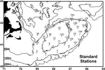 Figure 2. Locations where CTD data were collected. A
value of 100 was added to the Standard station number
where a SeaBird CTD cast was substituted for a Mark V
cast.
Figure 2. Locations where CTD data were collected. A
value of 100 was added to the Standard station number
where a SeaBird CTD cast was substituted for a Mark V
cast. scans of each variable exceed some preset limit. The "Smart Editor" within CTDPOST was then used to interpolate over the flagged values. The cleaned raw data were converted into pressure averaged 1 decibar files using algorithms provided by Robert Millard of WHOI, which had been adapted for use with the MK5.
The MK5 experienced an intermittent problem with its conductivity data channel. The instrument would work fine on one station, but on the next the conductivity signal would be very low, with values of around 0.3, rather then around 30. All of the other data channels appeared to function well throughout the cruise. Review of the raw conductivity data suggested that, when it occurred, the problem was that the high order bits of the conductivity signal from the instrument were missing. When the data appeared good, they compared quite well with the SBE19 data - and they are believed not to be degraded in quality. On the 11 stations where the problem occurred, the SBE19 data was substituted as the primary hydrographic data.
The locations of the MK5 casts made during the bank-wide survey are identified by the consecutive cast number (Figure 2 - numbers > 100 indicate that SBE19 data was substituted). The surface and bottom temperature and salinity distributions are shown in Figures 3 and 4. Surface and bottom anomalies of temperature and salinity as well as a stratification index (sigma-t difference from the surface to 30 meters) were calculated using the NMFS MARMAP hydrographic data set as a reference. The anomaly distributions are shown in Figures 5-7. The distributions of surface and bottom measured fluorescence are shown in Figure 8. Profiles of each MK5 CTD cast with a compressed listing of the preliminary data are found in Appendix C.
The volume average temperature and salinity of the upper 30 meters were calculated for the four sub-regions of the Bank shown in Figure 9. These values are compared with characteristic values that have been calculated from the MARMAP data set for the same areas and calendar days.
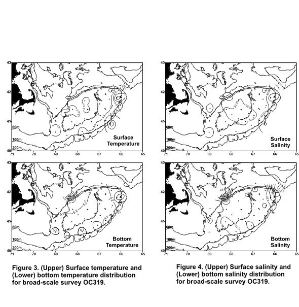
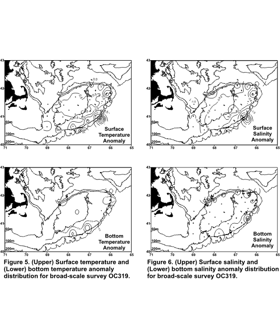
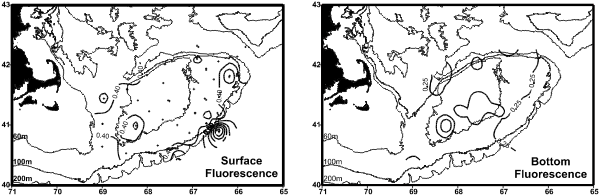 Figure 8. Surface and bottom fluorescence for broad-scale survey OC319
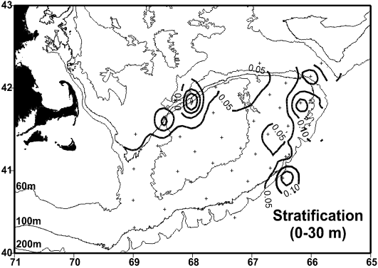 Figure 7. Stratification in the upper 30 m of the water column for broad-scale survey
OC319.
Figure 7. Stratification in the upper 30 m of the water column for broad-scale survey
OC319.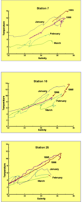 Figure 10. Temperature/salinity curves for
water properties in January, February and
March 1998 at (Top) Standard station 7,
(Middle) Standard station 16 and (Bottom)
Standard station 25. The curves for each
station in March 1995 and March 1996 are
also included as dashed line.
Figure 10. Temperature/salinity curves for
water properties in January, February and
March 1998 at (Top) Standard station 7,
(Middle) Standard station 16 and (Bottom)
Standard station 25. The curves for each
station in March 1995 and March 1996 are
also included as dashed line. The low salinity conditions observed in 1996 and 1997 have continued into 1998. The January 1998 survey results suggested that the salinity might be returning toward near ‘normal’ values, with anomalies less negative than observed in 1997. However, the anomaly values on the northern half of the Bank in February and again on this survey, listed in Figure 9, are about 0.5 salinity units lower than observed on the January 1998 survey and are comparable to the anomalies in 1997. The temperature anomalies on this survey are somewhat higher (warmer) than observed in other surveys since 1995.
Scotian Shelf water was observed along the southeastern edge of the Bank, as indicated by salinities < 32 and negative temperature anomalies. The suggestion, as with the February survey, was that an intrusion of Scotian Shelf water existed of the southern edge of the Bank. A satellite image received during the cruise did show a cold tongue of water extending from the Scotian Shelf to along the southern edge of the Bank.
The average fluorescence values (0-30 m depth) across the whole Bank in both the February and March surveys were the lowest observed in the GLOBEC broad-scale program ( 0.3 volts). These values are about half of those in the same months in 1997 and a third of the 1995 and 1996 values. A comparison of the chlorophyll values from the different cruises will be required before the significance of this decrease in average fluorescence can be determined.
Substantial changes in the properties of Slope Water off the southern flank of the Bank are indicated in the data from the three survey cruises this year. Figure 10 shows temperature-salinity plots for standard stations 7, 16, and 25 from the January, February and March surveys (solid lines). The March 1995 and 1996 data are also plotted (dashed lines). At salinities above 33.5 a progressive decrease in temperature occurred from January to March, particularly at station 7. This is not believed to be a seasonal change, but indication of the movement of colder fresher Slope Water into the region. At all three stations, the March curves were substantially colder than in 1995 and 1996. The March 1998 properties are similar to the colder Slope Water observed in the area during the 1960’s. A personal communication from K. Drinkwater (Bedford Institute of Oceanography) indicated that a similar change had been observed recently off the Scotian Shelf and that he expected it to arrive in the Northeast Channel/Georges Bank region around January - which seems to have occurred.
Zooplankton and Ichthyoplankton studies based on Bongo and MOCNESS tows.
(John Sibunka, Maria Casas, James Gibson, James Pierson, Rebecca Jones, Stephen Brownell, and Riley Young)
(1) Principle objectives of the ichthyoplankton group in the broad-scale part of the U.S. GLOBEC Georges Bank Program were to study the composition of the larval fish community on Georges Bank, to define larval fish distribution across the Bank and within the water column, to determine those factors which influence their vertical distribution, and to determine bank-wide versus "Patch-Study" mortality and growth rates. Emphasis in this study is on cod and haddock larvae along with their predators and prey. This study also includes larval distribution and abundance, and age and growth determination. These objectives were implemented through use of Bongo net and 1-m2 MOCNESS to make the zooplankton collections.
(2) The primary objective of the zooplankton group was to complete a bank-wide survey of Georges Bank to determine the distribution, abundance, and stage composition of the target species Calanus finmarchicus and Pseudocalanus spp. A second objective was to identify, quantify, and describe the occurrence of abundant non-target species in order to provide a description of the environment occupied by the target species. These objectives were implemented by using the 1-m2 MOCNESS, a vertically discrete, multiple opening and closing net system for sampling copepods and larger zooplankton, and submersible pumps for sampling the small, naupliar stages.
In addition to these objectives, the zooplankton group was responsible for obtaining
sub-samples from the 1-m2 MOCNESS hauls for population genetic studies of Pseudocalanus spp. to be completed by Dr. A. Bucklin at the University of New Hampshire.
Finally, an additional 1-m2 MOCNESS tow was completed at Station 38 to collect live C. finmarchicus for Dr. William Macy at the Graduate School of Oceanography/University of Rhode Island for an ongoing herring feeding experiment and Limacina retroversa for Dr. Scott Gallager (WHOI) for laboratory experimental studies.
Bongo tows were made with a 0.61-m frame fitted with paired 335 μm mesh nets. A 45 kg ball was attached beneath the Bongo frame to depress the sampler. Digital flow meters were suspended in the mouth of each net to determine the volume of water filtered. Tows were made according to standard MARMAP procedures, (i.e., oblique from surface to within five meters of bottom or to a maximum depth of 200 m while maintaining a constant wire angle throughout the tow). Wire payout and retrieval rates were 50 m/min and 20 m/min respectively. These rates were reduced in shallow water (<60 m) to obtain a minimum of a five minute tow or reduced due to adverse weather and sea conditions. A SeaBird CTD was attached to the towing wire above the frame to monitor sampling depth in real time mode and to measure and record temperature and salinity. Once back on board, the 335 μm mesh nets were rinsed with seawater into a 330 μm mesh sieve. The contents of one sieve were preserved in 5% formalin and kept for ichthyoplankton species composition, abundance and distribution. The other sample was preserved in 95% ethanol and kept for age and growth analysis of larval fish. The same preservation procedure was followed as for the 1-m2 MOCNESS.
At stations where the 1-m2 MOCNESS system could not be used due to adverse weather conditions, a second Bongo tow was made. This frame was fitted with both 335 μm mesh and 200 μm mesh nets. Digital flow meters were suspended in the mouth of each net to determine the volume of water filtered. Tows were made according to standard MARMAP procedures except maximum tow depth was 500 m. Wire payout and retrieval rates were 50 m/min and 20 m/min respectively. The nets were each rinsed with seawater into a corresponding mesh sieve. The 200 μm mesh sample was retained for zooplankton species composition, abundance, and distribution, and preserved in 10% formalin. The other sample (335 μm mesh) was kept for molecular population genetic analysis of the copepod, Calanus finmarchicus, and preserved in 95% ethanol. After 24 h of initial preservation, the alcohol was changed.
The 1-m2 MOCNESS sampler was loaded with ten nets. Nets 1-4 were fitted with 150 μm mesh for the collection of older and larger copepodite and adult stages of the zooplankton. Nets 0, and 5-9 were fitted with 335 μm mesh for zooplankton (nets 0 and 5) and ichthyoplankton (nets 6-9) collection. Tows were double oblique from the surface to within 5 m from the bottom. The maximum tow depth for nets 0, 1 and 5 was 500 m, and for net 6 was 200 m (if net 5 was sampled deeper than 200 m, it was returned up to 200 m and then closed). Winch rates for nets 0-5 were 15 m/min and for nets 6-9, 10 m/min. For those nets fished >200 m, the decent rate was increased so that the maximum vertical velocity of the MOCNESS was 25 m/min. This was providing the net angle did not go below 25° and the net horizontal speed did not drop below 0.5 kts. The depth strata sampled were 0-15 m, 15-40 m, 40-100 m, and >100 m. The first (#0) and sixth (#5) nets were integrated hauls. For shallow stations, with only 2 or 3 of the depth strata, not all nets were fished. The contents of nets 0-4 were sieved through 150 μm mesh sieve, sub-sampled using a 2-L plankton sample splitter if the final biomass volume was too large for one quart jar, and then preserved in 10% formalin. Samples from nets 5-9 were sieved through 330 μm mesh sieve and preserved in 95% ethanol. After 24 h of initial preservation, the alcohol was changed. The used ethanol was retained for disposal or recycling ashore. At priority 1 and 2 stations, 90-ml sub-samples from the 150 μm mesh nets were removed and preserved in 10% formalin for Dr. Charles Miller (OSU). In addition, at priority 1 and 2 stations, 90-ml sub-samples from these same nets were removed and preserved in 95% ethanol. These samples were collected for Dr. Ann Bucklin for population genetic studies to distinguish the Pseudocalanus species found on Georges Bank.
The 10-m2 MOCNESS was loaded with five 3.0 mm mesh nets. Tows were oblique from surface to ~10 m from bottom or a maximum depth of 500 m. The same depth strata were sampled as with the 1-m2 MOCNESS. The winch rate for retrieval varied between 5 and 15 m/min depending on the depth stratum. The slow winch rates were used in order to filter at least 4,000-5,000 m3 of water per depth stratum sampled. A stepped oblique tow profile during retrieval was used to achieve this, if needed. Catches were sieved through a 335 μm mesh, and preserved in 10% formalin.
The Pacer high-volume pump was used to collect nauplii and younger, smaller copepodite stages of zooplankton. The intake hose was deployed off the starboard side hydro boom by connecting the intake end, fitted with a 1.7-L Niskin bottle cut in half lengthwise, to the winch wire. The boom winch meter block was zeroed at the surface and the wire out reading was used to determine the depth of the cast. A 70 kg weight was used to depress the array. Three or four 30-m sections of 7 cm diameter hose were connected to the pump (depending on the depth of the station), allowing the intake hose to attain a maximum depth of approximately 117 m. At shallow stations, the intake hose nozzle was lowered to 3 meters off the bottom. Integrated depth samples were collected with 35 μm mesh nets, sieved through a 30 μm mesh sieve and preserved in 10% formalin. At stations with a maximum sampling depth of more than 85 m, samples were taken from the maximum depth to 75 m, 75-40 m, 40-15 m, and from 15 m to surface. At stations with a maximum sampling depth of less than 85 m, samples were taken from the maximum depth to 40 m, 40-15 m, and 15 m to surface. Before samples were collected, water was diverted from the net and the hose was allowed to flush completely, to assure that the zooplankton from the desired strata were obtained. At the last depth interval, the intake section was held just below the surface for 51 or 88 s (when three or four hose sections were used, respectively) allowing the sample to pass completely through the hose. Wire retrieval rate was approximately 4 m/min. This rate was used to obtain volumes of 500 L per 5 m depth interval sampled.
To collect Calanus finmarchicus for the live herring feeding experiments, the 335 μm mesh nets were used on the 1-m2 MOCNESS. The animals caught in the cod end buckets were gently released into 30-gallon plastic trash cans previously filled with seawater using the Pacer pump system.
Preliminary Summary of Zooplankton Findings.
(Maria Casas, Jennifer Crain, Jim Gibson, Jamie Pierson, and Riley Young)
Preliminary observations were made from the samples collected using the 1-m2 MOCNESS. Calanus finmarchicus (Figure 11A) was widespread throughout the Bank. All developmental stages were seen with a propensity toward younger stages, although adult females and males were also abundant. Pseudocalanus spp. was also present, if not abundant, at most stations. Highest concentrations were seen at stations 26, 27, and 33. Scatterings of Centropages typicus and C. hamatus were observed at most of the stations sampled.
Hydroids (Figure 11B) were abundant at many of the stations within the 60 meter isobath. This presence of hydroids seems to be earlier than usual this season compared to previous years.
Fish eggs and larvae (Figure 11C, D) were seen at most stations on and around the bank (see the preliminary findings of the Ichthyoplankton Group).
The presence of larvaceans (Figure 11E) and their houses at numerous stations around the bank led to a wealth of amorphous mucous, sometimes thick enough to clog the nets.
The pteropod Limacina (Figure 11F) was seen in patchy layers at various stations in lesser abundance than in the January broad-scale cruise.
Observations of zooplankton species composition were made at most Standard stations sampled during this cruise. These observations were made from the net #0 samples (335 μm mesh), 1-m2 MOCNESS, unless otherwise stated. Brief descriptions appear in Appendix 2, part1.
Samples Collected by the Zooplankton and Ichthyoplankton Groups:
Gear Tows Number of Samples
1. Bongo nets, 0.61-m 79 tows 76 preserved, 5% formalin
335-μm mesh 79 preserved, EtOH
200-μm mesh 2 preserved, 10% formalin
2. MOCNESS, 1-m2 38 tows
150-μm mesh (Nets 1-4) 118 preserved, 10% formalin
335-μm mesh (Net 0) 38 preserved, 10% formalin
335-μm mesh (Nets 5-9) 153 preserved, EtOH
3. MOCNESS, 10-m2 14 tows
3.0-mm mesh 52 preserved, 10% formalin
4. Pump 19 profiles
35-μm mesh 60 preserved, 5% formalin
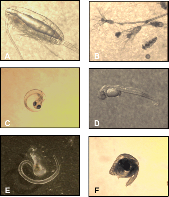 Figure 11. Video images of zooplankton collected on OC319. A) The copepod, Calanus
finmarchicus. B) Hydroids. C. An “eyed” gadid egg. D. A cod fish larva. E. A
larvacean. F. The pteropod, Limacina retroversa.
Figure 11. Video images of zooplankton collected on OC319. A) The copepod, Calanus
finmarchicus. B) Hydroids. C. An “eyed” gadid egg. D. A cod fish larva. E. A
larvacean. F. The pteropod, Limacina retroversa.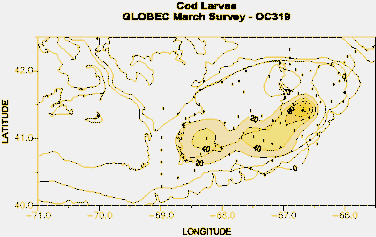 Figure 12. The distribution of larval cod/pollock based on
qualitative counts made while at sea on OCEANUS 319.
Figure 12. The distribution of larval cod/pollock based on
qualitative counts made while at sea on OCEANUS 319.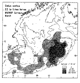 Figure 13. The Distribution of cod based on
samples collected during the MARMAP Program
(1977-1987).
Figure 13. The Distribution of cod based on
samples collected during the MARMAP Program
(1977-1987).Preliminary Summary of Ichthyoplankton Findings.
( John Sibunka, Rebecca Jones, and Stephen Brownell)
The samples collected at 40 GLOBEC broad-scale stations from both the Bongo and 1-m2 MOCNESS and from the Bongo at the intermediate stations, were examined on shipboard for the presence of fish eggs and larvae. The samples were preserved, and observed while in the jar with the aid of a magnifying glass. This was done in an attempt to obtain a qualitative estimate of abundance, distribution, and size range of ichthyoplankton on Georges Bank. The following observations are based on examination of samples in the jars following preservation. The formalin-preserved samples are clearer, and delicate eggs are less likely to collapse than those preserved in ethanol.
Cod (Gadus morhua) and/or Pollock (Pollachius virens):
Larval cod/pollock (microscopic
observation is required for separation and
positive identification between the two
species) dominated the catches in both
abundance and occurrence of larval fish
collected this cruise. Their distribution
ranged virtually across the entire length of
Georges Bank (Figure 12). The maximum
size range of these larvae were from 3-25
mm in length, with most measuring
between 5-10 mm. The largest collections
of cod/pollock larvae were made in the
south-central area. The greatest catch of
cod/pollock larvae for this cruise occurred
at Standard station 18, where an estimated
number of 160 individuals were collected.
The length of the larvae at this station
ranged from 3-8 mm. The distribution of
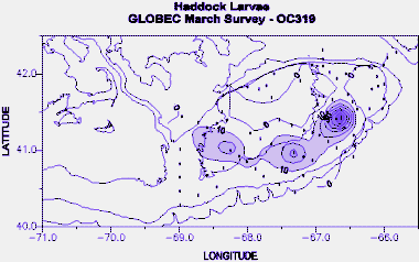 Figure 14. The distribution of larval haddock based on
qualitative counts made while at sea on OCEANUS 319.
Figure 14. The distribution of larval haddock based on
qualitative counts made while at sea on OCEANUS 319.
cod/pollock larvae collected on this cruise is the most extensive and the abundance estimates the largest when compared to the results from the previous three year broad-scale surveys for the month of March (refer R/V ENDEAVOR No.263, R/V OCEANUS Nos. 275 and 300 cruise reports). It is also the largest occurrence of cod/pollock larvae reported from any of the broad-scale surveys to date.
The month of March generally denotes the end of the pollock spawning season. If we then assume that most, if not all, of these larvae are cod and compare the results of this cruise to the historical NEFSC MARMAP data for cod larvae (size range 2.5-5.4 mm length) on Georges Bank for the month of March, we see a striking similarity in both distribution and the area of maximum abundance (Figure 13). Note that the abundance of cod larvae represented in the MARMAP figure are for the number of larvae per 10-meter2, whereas the figure depicting the abundance of cod on this survey are for unadjusted numbers of larvae collected.
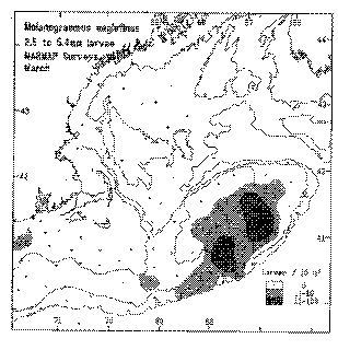 Figure 15. The Distribution of haddock based on
samples collected during the MARMAP Program
(1977-1987).
Figure 15. The Distribution of haddock based on
samples collected during the MARMAP Program
(1977-1987).Haddock (Melanogrammus aeglefinnus):
Haddock larvae (size range 3-15 mm; most ≤ 6 mm length) were collected in small to moderate numbers from the western area of Georges Bank eastward across the south central and northern portion of the Bank. None were caught in the central and southern sector of the Northeast Peak region of the Bank (Figure 14). The largest catches of haddock were made in the south central portion of the Bank where an estimate of 40 larvae (size range 4-10 mm length) was made at station 9 and 110 larvae (size range 3-4 mm length) were collected at station 18. This distribution pattern is similar to that of the cod/pollock collected during this survey. The estimated abundance of larval haddock collected during this cruise is the largest of any previous broad-scale survey completed in the past three years. A comparison of the larval haddock catch results of this cruise to the historical NEFSC MARMAP data for haddock larvae (size range 2.5-5.4 mm length) on Georges Bank for the month of March, shows a strong resemblance in both distribution and areas of abundance (Figure 15). Note that the haddock larvae represented in the MARMAP figure are for the number of larvae per 10-meter2, whereas the figure depicting the abundance of haddock larvae on this survey are for unadjusted numbers of specimens collected.
Sand lance larvae (maximum size range 10-50 mm in length, with most between 18-30 mm ) appeared to be concentrated along the entire northern area of Georges Bank where a large catch of about 110 larvae (size range 30-50 mm length) were collected at standard station 30. Larval sand lance were also collected intermittently across the central and northern portion of the Bank. The numbers of sand lance in this area of the Bank were small except at intermediate Bongo stations 42 and 61 where an estimated 75 and 50 larvae were caught respectively, and at standard station 30 where there was a catch of about 100 larvae. Compared to the results from the March 1997 cruise (refer R/V OCEANUS No. 300 cruise report) sand lance larvae collected on this survey were similar in size, but were more restricted in distribution and lower in estimated abundance numbers. The sand lance larvae collected in March 1997 dominated the catches in both abundance and occurrence of fish larvae collected on that cruise.
 Figure 16. The distribution of gadid eggs based on
qualitative counts made while at sea on OCEANUS 319.
Figure 16. The distribution of gadid eggs based on
qualitative counts made while at sea on OCEANUS 319.Cod/haddock/pollock eggs observed in the plankton samples collected on the cruise were mainly concentrated in the south central to the Northeast Peak area of Georges Bank. The largest catches of several hundred eggs per station were made in the Northeast Peak region. Small and intermittent catches of large size gadoid eggs were made in the south- east central, east portion and north western area of the Bank (Figure 16). Although the distribution of large gadoid eggs is similar to the results reported for the March 1997 broad-scale survey (refer R/V OCEANUS No. 300 cruise report) the estimated abundance values of eggs seen in the samples was noticeably smaller.
The following fish larvae were also identified in the ichthyoplankton samples collected during this broad-scale survey.
1. Atlantic herring Clupea harengus
2. Sculpin Myoxocephalus sp.
3. Lanternfish Myctophidae
4. Sea raven Hemitripterus americanus
5. Rock gunnel Pholis gunnellus
6. Wolf fish Anarhichas sp.
Preliminary Summary of the 10-m2 MOCNESS samples.
(Rebecca Jones and Maria Casas)
The samples collected from 10-m2 MOCNESS were examined on shipboard for a qualitative estimate of abundance, distribution, and size range of both the invertebrate and the fish community at station. These observations are presented in Appendix 2, part 2.
Microzooplankton Analysis. The Importance of Microzooplankton in the Diet of Newly Hatched Cod Larvae: Broad-scale Studies of Prey Abundance.
(Stephanie Innis and Jennifer Crain for Scott Gallager)
One objective of this study is to characterize seasonal changes in the potential prey field for newly hatched cod larvae with respect to prey motility patterns and the prey size spectrum.
Prey Size, Abundance and Motility Experiments Purpose: To observe, record, and analyze motility patterns and size spectrum of available prey from three locations in the water column- near bottom, pycnocline, and upper well-mixed area at all broad- scale stations from January through June.
General Procedure: Water samples were collected from the near bottom, and pycnocline areas of the water column using Go-Flo bottles on the Neil Brown Mark V CTD. Surface samples were collected with a plastic bucket. Go-Flo bottle samples were collected by gently siphoning from the top of the bottle instead of the normal port so that microplankton were not disrupted. Tissue culture flasks (200-ml) were filled after being dipped in soapy water and air dried to prevent fogging. To further prevent fogging as well as maintaining a constant low temperature, flasks were transferred to an incubator at 5° C immediately after filling.
Each flask, in turn, was placed in a holder across from a B/W high-res Pulnix camera fitted with a 50 mm macrolens and directly in front of a fiber optic ring illuminator fitted with a far-red filter. This apparatus was suspended within the incubator by a bungee cord to reduce vibration produced by the ship. Recordings were made using a Panasonic AG1980 video recorder with SVHS formatted cassettes, a Panasonic TR-124MA Video Monitor, and a timing device for a period of 15 minutes for each sample. The flask was then replaced with the next sample and recordings continued. The field of view was calibrated for each videotape by focusing on the front and back of a flask, and recording the width and height of the filed of view. For recording, the focus was adjusted to the middle of the flask. The depth of field was set to ~2.5 for the first eight consecutive stations (3,4,7,9,12, 13,16,17) and then set to 8+ for the remainder of the cruise, in order to maximize the field of view.
Priority #1 stations were analyzed; samples were recorded and preserved in 10% Lugols solution. Water samples from priority #2 stations were recorded, but not preserved. Microzooplankton samples from station 12 (priority #1) and station 25 (priority #2) were NOT collected and analyzed because these fell during the opposite watch, and time restraints did not allow anyone to fit in the recordings.
Motility patterns will be analyzed with the Motion Analysis EV system. The final output will be particle size distribution and a motility spectra associated with each particle. This will be compared with species composition in the microzooplankton fraction preserved in Lugols solution.
(Jennifer Crain and Charles B. Miller)
We have observed that Calanus juveniles which are preparing for diapause tend to have smaller, less developed gonads than those in the process of maturing directly into adults. In May of 1997, the first sampling of our gonad development series, small, undifferentiated gonads were typical among C5's examined. By contrast, in January of 1998, as the recently emerged resting stock of C5's was getting ready to molt into adults, nearly every individual sampled had a large, well-developed gonad, often with the oviducts easily distinguishable. Most of these animals were recognizably female, with only one or two gonads identified as possible testis. Observations of C5 gonads from the February cruise were virtually identical to those made in January.
Now the Calanus G1 generation is maturing, and C. finmrchicus is clearly the dominant zooplankter both on and near Georges Bank. Egg-laden females from the G0 generation still dominate the adult population, although adult males are also present, especially in the deeper samples. Nauplii and copepodites (stages C1 through C5) were seen at all stations. Live sorting of sub-samples from deep and shallow nets at standard stations 3, 4, 9, 18, 23, 39, 27, 35 and 38 yielded plenty of healthy C5s for gonad examinations. Observations on the developmental status and length of each animal's gonad were made. As in January and February, almost all of the fifth copepodites had large, well developed gonads. A portion (approximately 15%) of these were in the early stages of gonad development, when the gonad is small (approximately 0.32 to 0.60 mm) and has not yet begun to differentiate. The majority (approximately 45%) of the gonads examined were ovaries complete with developing oviducts, but a significant proportion (approximately
 Figure 17. (Top) Male C. finmarchicus.
(Bottom) Female C. finmarchicus.
Figure 17. (Top) Male C. finmarchicus.
(Bottom) Female C. finmarchicus.15%) were identified as possible maturing testes. Developing testes (see Figure 17a) look similar to developing ovaries (Figure 17b), and are characterized by a much blockier overall shape, conforming less to the dorsal contour of the oil sac and smaller cell size. An early stage testis begins forming two anteriorly directed ducts which are homologous with the oviducts of a female copepod. As the development progresses, the right duct degenerates while the left one turns downward and backward to become the vas deferens. Several individuals were seen with vas deferens clearly developed, but most of the suspected males were identified on the basis of overall gonad appearance, and will need to be confirmed in the lab using differential interference contrast microscopy. The proportion of probable male C5's was far higher on this cruise than on any previous cruises, and is assumed to reflect males being recruited into the G1 generation.
On broad-scale cruise OC319, we continued to gather data on correlations between gonad development, oil sac volume, and tooth phase in Calanus finmarchicus fifth copepodites. An image of each individual C5 examined was captured and oil sac volumes were calculated from areal measurements using image analysis software. Each animal was individually preserved in formalin for later verification of field observations of the gonads using differential interference contrast microscopy. Correlations between gonad development and oil sac volume will be assessed with respect to relative age-within-stage, as evidenced by tooth phase.
We also continued to collect formalin-preserved sub-samples from the 150 micron-mesh 1-m2 MOCNESS nets at all priority 1 and 2 stations for ongoing studies of jaw phase distributions and possible secondary environmental sex determination in Calanus finmarchicus. Ethanol-preserved sub-samples were taken from 1-m2 MOCNESS net 5 at the same stations, to be used for molecular determination of the underlying genetic sex of individual Calanus.
Phytoplankton chlorophyll, nutrients and light attenuation studies.
(David W. Townsend, Jiandong Xu)
Water samples were collected during the March 1998 R/V OCEANUS broad-scale survey cruise to Georges Bank for the analysis of:
∙ dissolved inorganic nutrients (NO3+NO2, NH4, SiO4, PO4);
∙ dissolved organic nitrogen and phosphorus;
∙ particulate organic carbon, nitrogen and phosphorus, and
∙ phytoplankton chlorophyll a and phaeophytin
These results will be posted on our web site (http://grampus.umeoce.maine.edu/globec/globec.html) as soon as they become available.
Collections were made at various depths at all of the regular hydrographic stations sampled during the March 1998 broad-scale survey cruise aboard R/V OCEANUS, using the 1.7 liter Niskin bottles mounted on the rosette sampler. Additional surface water samples were collected at positions between the regular stations using a Kimmerer Bottle to sample a depth of 2 m.
Light attenuation of photosynthetically active radiation (PAR) was measured at several stations at or about noon when sea state conditions allowed. A LiCor underwater spherical quantum sensor and deck-mounted cosine quantum sensor were used to compare the underwater light field as a function of depth and coincident surface irradiance.
Samples for dissolved inorganic nutrients and chlorophyll were collected at all stations (full and intermediate). Water samples for DIN were filtered through 0.45 μm Millipore cellulose acetate membrane filters, and the samples frozen immediately in 20ml polyethylene scintillation vials by first placing the vials in a seawater-ice bath for about 10 minutes. Samples will be analyzed on shore immediately following the cruise using a Technicon II 4-Channel AutoAnalyzer.
Water samples (50 mls) for dissolved organic nitrogen, and total dissolved phosphorus were collected at 2 depths (2 and 20 m) at each of the main stations and frozen as described above. These samples will be analyzed ashore using a modification of the method of Valderrama (1981).
Samples for particulate organic carbon and nitrogen were collected by filtering 500 mls from 2 depths (2 and 20 m) at each of the main stations onto pre-combusted, pre-ashed GF/F glass fiber filters, and filters frozen for analysis ashore. The filters will be fumed with HCl to remove inorganic carbon, and analyzed using a Control Equipment Model 240-XA CHN analyzer (Parsons et al., 1984).
Samples for particulate phosphorus were collected as for PON (but 200 mls will be filtered) and frozen at sea. Laboratory analyses will involve digesting the sample in acidic persulfate and then analyzing for dissolved orthophosphate.
Phytoplankton chlorophyll a and phaeopigments were measured on discrete water samples collected at all stations and determined fluorometrically (Parsons et al., 1984). The extracted chlorophyll measurements involved collecting 100 ml from all bottle samples taken at depths shallower than 60 m, filtering through GF/F filters, and extracting the chlorophyll in 90% acetone in a freezer for at least 12 hours. The samples were analyzed at sea using a Turner Model 10 fluorometer. These data will be used in regressions against measurements of in situ fluorescence as part of the regular CTD casts.
Parsons, T.R., Y. Maita and C.M. Lalli. 1984. A Manual of Chemical and Biological Methods for Seawater Analysis. Pergamon, Oxford. 173 pp.
Valderrama, J.C. 1981. The simultaneous analysis of total nitrogen and total phosphorus in natural waters. Marine Chemistry 10: 109-122.
(Peter Wiebe and Karen Fisher)
The primary focus of the bioacoustical effort on this cruise was to make high resolution volume backscattering measurements of plankton and nekton throughout the Georges Bank region on two frequencies, 120 kHz and 420 kHz. This was the second broad-scale cruise completed this year and followed the one in January. The acoustical data are intended to provide acoustical estimates of the spatial distribution of biomass of acoustical targets which span the size range of the target species (cod, haddock, Calanus, and Pseudocalanus) and their predators. Work on this cruise was designed to provide intensive continuous acoustic sampling along all the shipboard survey track lines in order to cover the entire Georges Bank region and was carried out successfully. The spatial acoustical mapping is also intended to provide a link between the physical oceanographic conditions on the Bank and the biological distributions of the species as determined from the net collections at the stations distributed throughout the Georges Bank region. One of our hypotheses is that continuous acoustic data between stations can be used to identify continuity or discontinuity in water column structure which can in turn be used to qualify the interpretation of biological and physical data based on the point source sampling.
On this cruise, a van located on the aft portion of the 01-deck on the R/V OCEANUS was the operations center for the high frequency acoustics work that was being done in an attempt to map the distribution and abundance of the animals living in the water column. The “acoustics system” consisted of the “Greene Bomber”, the chartreuse five-foot V-fin towed body, a Model 244 Hydroacoustics Technology, Inc Split-Beam Digital Echo Sounder (HTI-DES), several computers for data acquisition, post processing, and logging of notes, plus some other gear. In the Greene Bomber, there were two down-looking transducers (120 and 420 kHz each with 3 degree beams), and an Environmental Sensing System (ESS). The transducers were connected to
 Figure 18. BIOMAPER II and Greene
Bomber launch and recovery J-Frame
Figure 18. BIOMAPER II and Greene
Bomber launch and recovery J-Framea “MUX” bottle which provided the circuitry to multiplex the data coming from the transducers and transmit them to the echo sounder. The MUX bottle and the electrical cable were delivered just in time to be used for the first time on this cruise. The ESS was mounted inside the V-fin with temperature, conductivity, and fluorescence sensors attached to a stainless steel framework outside of the fiberglass housing. A downwelling light sensor was attached to the tail. The fish was also carrying a transponder that would have proved useful in locating it if it had happened to break free of the towing line.
 Figure 19. Acoustic measurements were made in all
areas of Georges Bank along the tracklines indicated
by the line connecting the Standard stations
locations.
Figure 19. Acoustic measurements were made in all
areas of Georges Bank along the tracklines indicated
by the line connecting the Standard stations
locations.The tow-body was deployed from the port quarter of OCEANUS. A new handling system was used on this cruise for the first time which consisted of a surplus hydraulically operated J-frame and winch (Figure 18) that had been reconstructed for this cruise. In addition, there was a power pack to supply the hydraulic power to drive the J-frame and winch. The J-frame when fully lowered over the side of the vessel, allowed the Greene Bomber to be deployed about 3 meters away from the vessel. A flexible 1" (2.5 cm) diameter synthetic line (breaking strength ~ 40000 lbs) was used to tow the towed body. Separate electrical cables were used for power and communication to the transducers and environmental sensing packages in the towed body. Data were collected both during and between stations. The general towing speed was 7.0 to 8 knots. The echo sounder collected data at two pings per second per frequency. Conditions for conducting an echo sounder survey of the Bank were quite variable during this cruise with conditions being poor during the windy periods and quite good during less windy periods. We were able to collect acoustics data along essentially the entire trackline of the cruise. The length of trackline acoustically mapped was ~726 nm (Figure 19; Table 1).
In the van, the data came in on the electrical conductors from each transducer and from the ESS through the MUX bottle in the Greene Bomber. The van based HTI-DES has its own computer and five digital Signal Processor boards (DSPs). It received the data from the transducers, did a series of complex processing steps, and then transferred the results to a Pentium PC over a local area network (LAN) where the data were logged to disk and displayed. The “raw” unprocessed data were also written to a DAT tape (each tape holds two gigabytes of data and we used about 100 tapes during this cruise). Immense amounts of data were handled very quickly by this system. The environmental data came into a second PC and were processed, displayed, and logged to disk. Both systems required GPS navigation data and those data were being supplied by the ship’s P-code GPS receiver and a Rockwell receiver that we put together. Periodically, the data were transferred to another Pentium PC computer for post-processing. It was at this stage that we could visualize the acoustic records and begin to see the acoustic patterns which were characteristic of the Bank. Additional post-processing of the data was also done on a Pentium Pro PC.
Greene Bomber Recovery In a Gale
As described in the narrative, we began collecting data on March 16, after sampling was completed at the third station ( 41). Gale force winds and building seas forced us to cease work and batten down the equipment in preparation to ride out the storm on 21 March mid-way between Stations 22 and 24. As part of the preparation, we decided to bring the Greene Bomber back on board. Karen Fisher and Peter Wiebe shut the acoustic and the ESS system off. Wiebe and others suited up to brave the elements. The Bosun had specified that only four individuals were to participate in the recovery. The air was cold, the wind chill pretty fierce, and the main deck awash. The plan was to have Wiebe operate the J-frame and winch, Jamie Pierson and Horace Mediros handle tugger lines, and Jeff Stolp (the Bosun) direct the operation. With Stolp, Mediros, Pierson, and Wiebe on deck to bring the system in, Wiebe pushed the start button on the hydraulic power pack and nothing happened. Stolp suggested that the electrical circuits might be shorted. Wiebe got Patrick Mone, the chief engineer, to check out the circuit panel in the aft winch room where the power is sent to the power pack and he found the circuit breaker thrown. He reset it and Wiebe went back to the deck to try to start the power pack again. A low noise came out of the power pack's circuit panel as if it were trying to start, but nothing happened and then the noise disappeared. Mone went down to look at the circuit box in the winch room and as we were standing on the deck, the power pack's circuit panel box suddenly sparked. Stolp opened the circuit panel door slightly which released a puff of smoke and along with it the smell of cooked electrical parts. Mone appeared on the deck and it was clear that something in the box had shorted when he had reset the ship's circuit breaker turning the power on again.
It was much too rough and wet to think about opening up the power pack panel to see if the could be repaired. We were done trying to get the fish in by powering up the J-frame and winch. We started to talk about other ways to bring the fish aboard or to leave it in and have it ride out the storm. Wiebe chose not to let it ride out the storm - he didn't want the worry about the possibility of losing it nor did he want to chance fate again (another system, BIOMAPER, was lost on two very similar previous occasions in the same area). We could have used the capstan to pull in the towing cable since we had a kilim grip on the line with a thimble making for an easy attachment point. But the winch had a hydraulic brake which could not be released and thus the line could not be just pulled straight in. We set up a couple of the tuggers with snap hooks that could be used to hook onto the stainless steel framework around the fish once it was above the water, but we still needed a way to get it up out of the water. Putting a come-along on the towing line seemed iffy at best since we would have to pull in a bit, stop the line off, and then reset the come-along and bring in some more. During the time when the come-along was being reset, the fish would probably get creamed against the side of the ship.
Stolp went to the bridge to discuss the situation with the Captain and Mate. Wiebe went up a minute or two later with another idea which was to use the crane whip attached to a loop in the line going to the tail end of the fish to haul the fish up and move it over onto the deck. After a few minutes of discussion, it was decided to do this.
Down on the deck more hands arrived (Jim Gibson, John Sibunka, and Jim Lichter). Mediros operated the crane and moved it up and over to the port side, dropped the whip and ball/hook to where we could snap in the tail line. There was a need to put a loop in the tail line. Sibunka and Wiebe worked to put a loop in the tail line as close to the fish as possible. This was difficult because the fish was moving with the motion of the ship and the sea. As soon as we pulled the line in to make the loop, the fish would take it back. Sibunka put a couple of turns of the line around the rail to secure it and Wiebe tied the loop. We then passed the loop over to Stolp who put it on the whip's hook. Then Stolp motioned for Mediros to bring it up take up the whip and pull the fish to the sea surface where the tugger lines could be attached to the stainless steel rails on the fish. There was a slow down when it became clear that the tugger lines were not set up right. The seas were rolling and pitching the vessel and water was coming on board, but not too extremely. The fish was at the surface and occasionally came close to bashing into the hull, especially when a large sea came by. Stolp finally got the quick-release set up. Then it took several tries to get the first quick-release hook onto the fish. Finally it was hooked and tension was taken on that line. Raising the whip cable brought the fish up and more out of the water. During the time it took Gibson to get a second quick-release hook attached to the fish, a wave surged past and drove the fish into the hull options case first - the options case took a good part of the blow (but it survived and remained working). With the fish partially out of the water, but not clear of the rail, the tugger lines were pulled tight which spun the fish 180o and brought it against the hull again, but this time it brought the stainless steel bottom rails snug against the hull. Then, raising the crane boom raised the fish up above the bulwark rails and the tuggers pulled the fish inboard. The whip cable was lowered and the nose of the fish came to rest on the deck. With the rolling of the ship, it was a struggle to get the fish down on the deck in a position where it could be bolt-strapped to the deck. But finally it was there. What a relief to get it on board and in one piece. It took another 15 minutes to get all the lines straightened out and put away, and to get the electrical cables and towing line tied securely. The entire operation took about an hour.
The acoustic records showed a typical "well mixed" structure over a large fraction of the Bank (where the water column was well-mixed) and it was only on the outer margins of the Bank that the most variable acoustic patterns appeared. A section which had been surveyed repeatedly runs from between Standard stations 8 and 12 (Figure 20). This section is typical of the range of acoustic environments encountered on Georges Bank with strong stratification in the vicinity of the shelf/Slope Water frontal region where the water column is deepest and nearly homogeneous vertical structure on the crest of the Bank where water depths are shallower than 50-60 m. The 120 kHz and 420 kHz data sets while showing the same basic patterns, do differ in relative intensity both in the stratified and well-mixed portions of the acoustic section (Figure 20). An interesting feature was a “hole” in acoustic volume backscattering that occurred in the middle of the southern flank. Between stations 9 and 10, the volume backscattering dropped to quite low levels in the upper 30 meters (the lowest seen on the Bank this cruise) and they only picked up when we reached Station 10. Both frequencies displayed this feature, but it was most intense in the 120 kHz record.
Some of the acoustic structure seen along the outer margins of the southern flank of the Bank was caused by internal wave packets. There was a strong internal wave packet evident between stations 6 and 7 in about the same region that we have seen them in previous cruises. The acoustic records also showed some interesting patterns at Standard Station 9. The water at first sight seemed well mixed, but then we came across a fairly intense internal wave packet in the upper 40 m while doing the 10-m2 MOCNESS trawl (Figure 21). Internal waves must have some level of stratification in order to propagate and this fact made us take a closer look at the T/S data from the CTD and trawl. There was, indeed, temperature and salinity variations which were evident in the down and up-legs of the trawl tow trajectory which resulted in significant stratification in the upper 20 to 30 meters, the depth zone in which most of the wave was observed (Figure 22). Along the portion of the trackline from Station 5 to Station 10 that were in depths of 60 to 90 m, there were more "fish" targets than we have seen on past cruises. These were single individuals or clusters of individuals that positioned from just above the bottom to 20 or 30 meters above the bottom. Some of these strong "fish" targets were observed around Standard stations 5 and 6 in an otherwise homogeneous acoustic field. Coincidentally, there were quite a few fishing vessels in the areas between these two stations and the area out at the continental shelf break at Standard station 7.
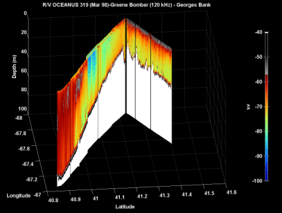
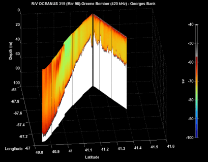 Figure 20. Along-track acoustics section running between
Standard stations 8 and 12 on the southern flank of Georges Bank.
(Top) 120 kHz data. (Bottom) 420 kHz data.
Figure 20. Along-track acoustics section running between
Standard stations 8 and 12 on the southern flank of Georges Bank.
(Top) 120 kHz data. (Bottom) 420 kHz data.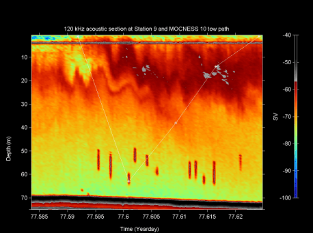 Figure 21. An acoustic section (120 kHz) through an internal wave packet
encountered during the 10-m2 MOCNESS trawl taken at Standard Station
9 on the southern flank of Georges Bank. The trajectory of the oblique
MOCNESS tow is indicated by the diagonal white line across the section.
The large individual targets below the intense scattering in the wave are
probably small fish schools, possibly herring.
Figure 21. An acoustic section (120 kHz) through an internal wave packet
encountered during the 10-m2 MOCNESS trawl taken at Standard Station
9 on the southern flank of Georges Bank. The trajectory of the oblique
MOCNESS tow is indicated by the diagonal white line across the section.
The large individual targets below the intense scattering in the wave are
probably small fish schools, possibly herring. 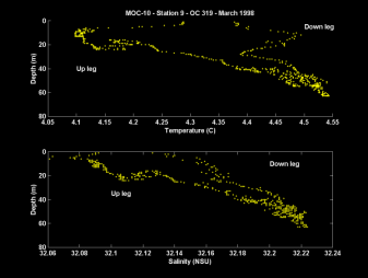 Figure 22. Temperature and salinity data collected on
the down and up-legs of the 10-m2 MOCNESS trawl
at Standard station 9.
Figure 22. Temperature and salinity data collected on
the down and up-legs of the 10-m2 MOCNESS trawl
at Standard station 9. Figure 23. Acoustic Sections (120 kHz) from Georges Bank into the Gulf of Maine basins.
A) Wilkinson Basin. B) Franklin Basin. C) Georges Basin.
Figure 23. Acoustic Sections (120 kHz) from Georges Bank into the Gulf of Maine basins.
A) Wilkinson Basin. B) Franklin Basin. C) Georges Basin.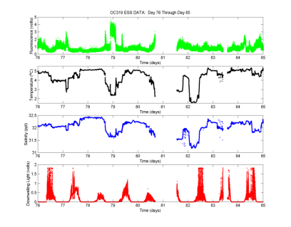 Figure 24. Greene Bomber along-track Environmental sensor data
collected at ~3 m depth.
Figure 24. Greene Bomber along-track Environmental sensor data
collected at ~3 m depth.There were three transect lines to and from the Bank to stations in the Gulf of Maine, one to Standard station 29 in Georges Basin, one to Standard station 34 in Franklin Basin, and one to Standard station 38 in Wilkinson Basin. There was a feature in common along each of these lines, namely the occurrence of an intense layering of volume backscattering in the deeper water along the margin of the Bank (Figure 23). In Wilkinson Basin the layer was patchy and the center of the intense scattering increased in depth in the transit from the Bank into the basin (Figure 23 A). In Franklin basin, the layer was not as intense, but still evident at depths around 100 m (Figure 23 B). In the Georges Basin section, the layer was most intense around 150 m and was embedded in what appeared to be an internal wave structure (Figure 23 C). This intense scattering was similar to that observed in the January broad-scale cruise (ALBATROSS IV cruise 9801). In both cases, a significant contributor to this scattering was the pteropod, Limacina retroversa. This species was quite abundant at depths where the intense scattering occurred and it is known that the shell of this animal is particularly efficient at backscattering high frequency sound.
Along track Environmental and ship MET Sensor Data
Surface temperature, salinity, and fluorescence values were gathered at 4 second intervals by the Environmental Sensing System (ESS) mounted on the Greene Bomber (Figure 24).
Throughout the record gathered by the ESS package on the Greene Bomber, temperature and salinity values tend to follow one another, with warmer saltier, or colder fresher waters being sensed following frontal crossings. A variety of distinct signatures were encountered in the surface waters, although all were quite cold (1.5 to 5.5o) and fresh (under 32.5 ppt).
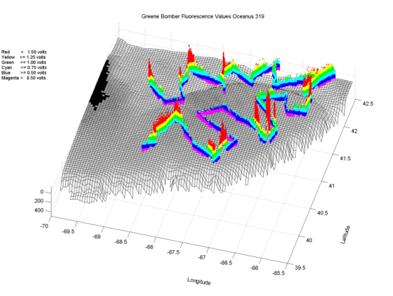 Figure 25. A 3-D view of the surface fluorescence data collected along the cruise track-line by a sensor on the Greene Bomber (OC319).
For the first half of the cruise, the trends of temperature and fluorescence tended to follow one another inversely, possibly indicating a substantial contribution of new production to the phytoplankton populations on the southern side of Georges Bank. A clear temperature front
was traversed when moving off the Bank, where temperatures dropped from the range of 4.7- 5.1o C down to 2.2-2.8o C. Fluorescence over the same front ranged from about 1 volt (+- 0.5 volts) in the warmer waters, to the 3-4.5 volt range (with 5 volts being the maximum on the fluorometer). From the beginning of the cruise until Greene Bomber came out of the water on Year-Day 80 during the storm, temperature and fluorescence seemed to show a relatively strong inverse covariance.
However, the second half of the cruise lacked this characteristic. In the very cold waters encountered, where temperature dropped to 1.5o C, fluorescence remained in the 1 volt range, even dropping slightly. Leaving this region, the water next encountered was warmer, but similar or even somewhat higher in fluorescence. The higher fluorescence values near this front were on the warmer side. Finally in the last two days, on the northern side of the Bank, 2 volt magnitude fluorescence fronts were evident in the absence of any significant change in temperature. On the final day, there was once again a fluorescence peak that coincided with a clear drop in temperature (Figure 24).
Atmospheric data were gathered by the IMET system on board R/V OCEANUS, and saved at both one minute, and one second intervals. Among the variables measured by the IMET system, were wind speed, barometric pressure, air temperature, and short wave radiation (Figure 26).
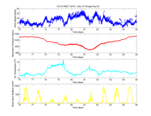 Figure 26. The OCEANUS along-track
meteorological data.
Figure 26. The OCEANUS along-track
meteorological data.The atmospheric data from the course of the cruise shows that the barometer fell from 1035 mbars to 990 mbars over a period of 5 days, starting on Day 76. Winds increased over the same period from around 10 knots to nearly 40 knots. Maximum air temperature (12o C) was reached the day before winds climbed to their maximum; air temperatures were between 0 and 5o C for the majority of the trip. Light levels dropped precipitously during the major weather change, with a series of three very dark cloudy days, and one fairly dark day before light levels returned to sunnier levels. The shape of the curves sensed by the ship mounted short wave radiation sensor, and the Greene Bomber mounted downwelling light sensor were similar.
As part of the physical oceanographic studies of the current structure and circulation on Georges Bank being conducted by R. Beardsley and R. Limeburner, GLOBEC Drifter Buoys are deployed at strategic locations periodically throughout the year to track the Lagrangian flow from the point of deployment. This drifter is constructed with a holey sock drogue (a Dacron cylinder 90 cm diameter by 3 m tall with 5 circular hoop stays) at the bottom connected by either a 10 m or a 40 m cable to a small float (18 cm diameter) which in turn is connected by about 2.6 m of cable to a larger spherical surface float (about 32 cm diameter). The surface float contains a sea surface temperature sensor, a GPS receiver, and an ARGOS satellite transmitter. Temperature, time, and position data are transmitted periodically to shore through the ARGOS telemetry system. On this cruise, three drifters were deployed. Single, ten-meter (shallow) drifters were released at stations 11, 27, and 33.
Shipboard ADCP (Acoustic Doppler Current Profiler) measurements.
The flow field over Georges Bank is driven by a complex set of forces. A primary factor is the strong semi-diurnal tides which dominate the high frequency variability (< 1 cpd) of the currents. Tidal rectification gives rise to a persistent sub-inertial clockwise circulation over the Bank. This circulation process can be substantially modified by the frequent storms common to the area, changes in the stratification of the Bank, and interactions with currents generated by offshore circulation features (i.e. Warm-Core Rings).
The Acoustic Doppler Current Profiler (ADCP) is one of the instruments being used to study the circulation processes on the Bank by C. Flagg and J. Candela. Water current measurements were obtained using an RDI ADCPs operating at 300 kHz. The 300 kHz system was operated continuously during the entire cruise. The transducers were mounted on the hull of the ship (5 m below the surface). The instrument was programmed to measure the current profile under the ship with a vertical resolution of 2 m, from 10 m depth to about 10 m from the bottom or up to a depth of about 120 m, whichever was shallower at a given location. The ADCP measures currents with respect to the ship. To obtain the water current with respect to the ocean bottom, the ship's motion needs to be removed from the current observations. The ship's motion will be removed using the bottom track (BT) velocity measured by the ADCP. Depending upon sea conditions, the ADCP can perform this operation in water depths shallower than 200 to 230 m. When the BT is lost, accurate navigation is used to remove the ship's velocity from the current.
The ADCP data collected on this cruise will be post-processed by Flagg and Candela.
1. Peter H. Wiebe Woods Hole Oceanographic Institution
2. David G. Mountain National Marine Fisheries Service, Woods Hole
3. John Sibunka National Marine Fisheries Service, Sandy Hook
4. Maria Casas University of Rhode Island
5. James Gibson University of Rhode Island
6. James Pierson University of Rhode Island
7. Riley Young University of Rhode Island
8. Rebecca Jones National Marine Fisheries Service, Narragansett
9. Stephen Brownell National Marine Fisheries Service, Narragansett
10. Jiandong Xu University of Maine
11. Karen Fisher Cornell University
12. Jennifer Crain Oregon State University
13. James Leichter Woods Hole Oceanographic Institution
14. Stephanie Anne Innis Woods Hole Oceanographic Institution
15. Michael Greene Oregon EPA Laboratory
16. Laura G. Stein S.S.S.G. Technician
1. Courtenay Barber, III Master
2. Anthony D. Mello Chief Mate
3. Emily McClure 2nd Mate
4. Jeffery M. Stolp Boatswain
5. Horace M. Medeiros AB
6. James R. Ryder AB
7. Michael Butler OS
8. Patrick S. Mone Chief Engineer
9. J. Kevin Kay Jr. Engineer
10. Alberto Collasius Jr. Engineer
11. Mitchell G. Barros Steward
12. Keith Massa Mess Attendant
|
|
|
|
|
LOCAL |
|
|
|
Water |
Cast |
|
|
|
||
|
Instr |
cast# |
Sta# |
Sta_std |
Mth |
Day |
hhmm |
s/e |
Lat |
Lon |
Depth |
Depth |
PI |
Region |
Comments |
OC07498.01 |
Depart |
|
|
|
3 |
15 |
1022 |
s |
4031.50 |
7040.50 |
5 |
0 |
Wiebe |
Broad-scale |
Depart Woods Hole, MA |
OC07598.01 |
BongoSB |
1 |
1 |
1 |
3 |
16 |
2 |
s |
4101.00 |
6859.40 |
85 |
79 |
Sibunka |
Broad-scale |
|
OC07598.02 |
BongoSB |
1 |
1 |
1 |
3 |
16 |
12 |
e |
4101.20 |
6859.40 |
86 |
79 |
Sibunka |
Broad-scale |
|
OC07598.03 |
MK5CTD |
1 |
1 |
1 |
3 |
16 |
25 |
s |
4101.30 |
6859.40 |
82 |
76 |
Mountain |
Broad-scale |
|
OC07598.04 |
MK5CTD |
1 |
1 |
1 |
3 |
16 |
56 |
e |
4101.30 |
6859.00 |
78 |
76 |
Mountain |
Broad-scale |
|
OC07598.05 |
MOC-1 |
1 |
1 |
1 |
3 |
16 |
113 |
s |
4101.00 |
6858.70 |
70 |
65 |
Durbin |
Broad-scale |
|
OC07598.06 |
MOC-1 |
1 |
1 |
1 |
3 |
16 |
144 |
e |
4100.10 |
6858.50 |
78 |
73 |
Durbin |
Broad-scale |
|
OC07598.07 |
BongoSB |
2 |
2 |
42 |
3 |
16 |
312 |
s |
4049.70 |
6859.70 |
76 |
72 |
Sibunka |
Broad-scale |
|
OC07598.08 |
BongoSB |
2 |
2 |
42 |
3 |
16 |
321 |
e |
4049.70 |
6859.90 |
74 |
72 |
Sibunka |
Broad-scale |
|
OC07598.09 |
BongoSB |
3 |
3 |
2 |
3 |
16 |
429 |
s |
4038.90 |
6859.50 |
66 |
60 |
Sibunka |
Broad-scale |
|
OC07598.10 |
BongoSB |
3 |
3 |
2 |
3 |
16 |
436 |
e |
4038.70 |
6859.70 |
65 |
60 |
Sibunka |
Broad-scale |
|
OC07598.11 |
MK5CTD |
2 |
3 |
2 |
3 |
16 |
445 |
s |
4038.50 |
6859.80 |
65 |
60 |
Mountain |
Broad-scale |
|
OC07598.12 |
MK5CTD |
2 |
3 |
2 |
3 |
16 |
453 |
e |
4038.20 |
6859.80 |
67 |
60 |
Mountain |
Broad-scale |
|
OC07598.13 |
MOC-1 |
2 |
3 |
2 |
3 |
16 |
509 |
s |
4037.70 |
6900.10 |
67 |
60 |
Durbin |
Broad-scale |
|
OC07598.14 |
MOC-1 |
2 |
3 |
2 |
3 |
16 |
532 |
e |
4037.40 |
6901.30 |
67 |
60 |
Durbin |
Broad-scale |
|
OC07598.15 |
BongoSB |
4 |
4 |
43 |
3 |
16 |
644 |
s |
4028.40 |
6859.60 |
77 |
70 |
Sibunka |
Broad-scale |
|
OC07598.16 |
BongoSB |
4 |
4 |
43 |
3 |
16 |
652 |
e |
4028.40 |
6900.00 |
77 |
70 |
Sibunka |
Broad-scale |
|
OC07598.17 |
SBCal |
1 |
4 |
43 |
3 |
16 |
704 |
s |
4028.30 |
6900.10 |
77 |
20 |
Mountain |
Broad-scale |
|
OC07598.18 |
SBCal |
1 |
4 |
43 |
3 |
16 |
707 |
e |
4028.30 |
6900.20 |
76 |
20 |
Mountain |
Broad-scale |
|
OC07598.19 |
BongoSB |
5 |
5 |
41 |
3 |
16 |
812 |
s |
4017.10 |
6859.40 |
97 |
90 |
Sibunka |
Broad-scale |
|
OC07598.20 |
BongoSB |
5 |
5 |
41 |
3 |
16 |
826 |
e |
4018.60 |
6859.70 |
97 |
90 |
Sibunka |
Broad-scale |
|
OC07598.21 |
MK5CTD |
3 |
5 |
41 |
3 |
16 |
842 |
s |
4018.60 |
6859.00 |
96 |
90 |
Mountain |
Broad-scale |
|
OC07598.22 |
MK5CTD |
3 |
5 |
41 |
3 |
16 |
851 |
e |
4018.50 |
6859.80 |
96 |
90 |
Mountain |
Broad-scale |
|
OC07598.23 |
MOC-1 |
3 |
5 |
41 |
3 |
16 |
907 |
s |
4018.60 |
6900.00 |
96 |
89 |
Durbin |
Broad-scale |
|
OC07598.24 |
MOC-1 |
3 |
5 |
41 |
3 |
16 |
939 |
e |
4019.80 |
6901.00 |
96 |
89 |
Durbin |
Broad-scale |
|
OC07598.25 |
GBomber |
1 |
5 |
41 |
3 |
16 |
1026 |
s |
4021.30 |
6900.40 |
85 |
4 |
Wiebe |
Broad-scale |
|
OC07598.26 |
BongoSB |
6 |
6 |
44 |
3 |
16 |
1310 |
s |
4025.10 |
6843.40 |
88 |
83 |
Sibunka |
Broad-scale |
|
OC07598.27 |
BongoSB |
6 |
6 |
44 |
3 |
16 |
1321 |
e |
4025.40 |
6843.50 |
87 |
83 |
Sibunka |
Broad-scale |
|
OC07598.28 |
GBomber |
1 |
6 |
44 |
3 |
16 |
1331 |
e |
4025.60 |
6843.60 |
86 |
4 |
Wiebe |
Broad-scale |
|
OC07598.29 |
GBomber |
2 |
6 |
44 |
3 |
16 |
1427 |
s |
4026.80 |
6840.70 |
84 |
4 |
Wiebe |
Broad-scale |
|
OC07598.30 |
BongoSB |
7 |
7 |
3 |
3 |
16 |
1628 |
s |
4031.70 |
6827.10 |
89 |
85 |
Sibunka |
Broad-scale |
|
OC07598.31 |
BongoSB |
7 |
7 |
3 |
3 |
16 |
1636 |
e |
4031.70 |
6827.00 |
89 |
85 |
Sibunka |
Broad-scale |
|
OC07598.32 |
Pump |
1 |
7 |
3 |
3 |
16 |
1653 |
s |
4031.70 |
6827.80 |
89 |
78 |
Durbin |
Broad-scale |
|
OC07598.33 |
Pump |
1 |
7 |
3 |
3 |
16 |
1732 |
e |
4031.70 |
6827.30 |
89 |
78 |
Durbin |
Broad-scale |
|
OC07598.34 |
MK5CTD |
4 |
7 |
3 |
3 |
16 |
1825 |
s |
4031.70 |
6828.00 |
89 |
84 |
Mountain |
Broad-scale |
|
OC07598.35 |
MK5CTD |
4 |
7 |
3 |
3 |
16 |
1837 |
e |
4031.80 |
6828.10 |
89 |
84 |
Mountain |
Broad-scale |
|
OC07598.36 |
MOC-1 |
4 |
7 |
3 |
3 |
16 |
1850 |
s |
4031.80 |
6828.30 |
89 |
80 |
Durbin |
Broad-scale |
|
OC07598.37 |
MOC-1 |
4 |
7 |
3 |
3 |
16 |
1917 |
e |
4032.30 |
6828.80 |
89 |
80 |
Durbin |
Broad-scale |
|
OC07598.38 |
MOC-10 |
1 |
7 |
3 |
3 |
16 |
2004 |
s |
4033.00 |
6829.50 |
82 |
70 |
Madin |
Broad-scale |
|
OC07598.39 |
MOC-10 |
1 |
7 |
3 |
3 |
16 |
2045 |
e |
4034.60 |
6830.70 |
75 |
70 |
Madin |
Broad-scale |
|
OC07598.40 |
BongoSB |
8 |
8 |
45 |
3 |
16 |
2314 |
s |
4046.10 |
6821.30 |
56 |
51 |
Sibunka |
Broad-scale |
|
OC07598.41 |
BongoSB |
8 |
8 |
45 |
3 |
16 |
2321 |
e |
4046.60 |
6821.60 |
56 |
51 |
Sibunka |
Broad-scale |
|
OC07698.01 |
BongoSB |
9 |
9 |
4 |
3 |
17 |
120 |
s |
4100.10 |
6815.10 |
54 |
50 |
Sibunka |
Broad-scale |
|
OC07698.02 |
BongoSB |
9 |
9 |
4 |
3 |
17 |
129 |
e |
4100.20 |
6815.30 |
55 |
50 |
Sibunka |
Broad-scale |
|
OC07698.03 |
Pump |
2 |
9 |
4 |
3 |
17 |
146 |
s |
4100.00 |
6815.40 |
54 |
52 |
Durbin |
Broad-scale |
|
OC07698.04 |
Pump |
2 |
9 |
4 |
3 |
17 |
230 |
e |
4059.40 |
6814.70 |
55 |
52 |
Durbin |
Broad-scale |
|
OC07698.05 |
MK5CTD |
5 |
9 |
4 |
3 |
17 |
235 |
s |
4059.30 |
6814.70 |
56 |
52 |
Mountain |
Broad-scale |
|
OC07698.06 |
MK5CTD |
5 |
9 |
4 |
3 |
17 |
246 |
e |
4059.10 |
6814.40 |
57 |
52 |
Mountain |
Broad-scale |
|
OC07698.07 |
MOC-1 |
5 |
9 |
4 |
3 |
17 |
258 |
s |
4059.00 |
6814.50 |
56 |
52 |
Durbin |
Broad-scale |
|
OC07698.08 |
MOC-1 |
5 |
9 |
4 |
3 |
17 |
322 |
e |
4059.00 |
6814.80 |
57 |
53 |
Durbin |
Broad-scale |
|
OC07698.09 |
MOC-10 |
2 |
9 |
4 |
3 |
17 |
354 |
s |
4059.10 |
6815.00 |
54 |
48 |
Madin |
Broad-scale |
|
OC07698.10 |
MOC-10 |
2 |
9 |
4 |
3 |
17 |
443 |
e |
4059.20 |
6815.20 |
54 |
48 |
Madin |
Broad-scale |
|
OC07698.11 |
BongoSB |
10 |
10 |
46 |
3 |
17 |
637 |
s |
4055.60 |
6807.50 |
58 |
53 |
Sibunka |
Broad-scale |
|
OC07698.12 |
BongoSB |
10 |
10 |
46 |
3 |
17 |
643 |
e |
4055.60 |
6807.60 |
59 |
53 |
Sibunka |
Broad-scale |
|
OC07698.13 |
SBCal |
2 |
10 |
46 |
3 |
17 |
646 |
s |
4055.70 |
6807.60 |
59 |
22 |
Mountain |
Broad-scale |
|
OC07698.14 |
SBCal |
2 |
10 |
46 |
3 |
17 |
650 |
e |
4055.70 |
6807.70 |
59 |
22 |
Mountain |
Broad-scale |
|
OC07698.15 |
BongoSB |
11 |
11 |
5 |
3 |
17 |
821 |
s |
4051.10 |
6800.10 |
63 |
56 |
Sibunka |
Broad-scale |
|
OC07698.16 |
BongoSB |
11 |
11 |
5 |
3 |
17 |
829 |
e |
4051.40 |
6800.60 |
63 |
56 |
Sibunka |
Broad-scale |
|
OC07698.17 |
MK5CTD |
6 |
11 |
5 |
3 |
17 |
839 |
s |
4051.60 |
6800.90 |
61 |
56 |
Mountain |
Broad-scale |
|
OC07698.18 |
MK5CTD |
6 |
11 |
5 |
3 |
17 |
848 |
e |
4051.70 |
6801.30 |
61 |
56 |
Mountain |
Broad-scale |
|
OC07698.19 |
MOC-1 |
6 |
11 |
5 |
3 |
17 |
859 |
s |
4051.70 |
6801.70 |
61 |
50 |
Durbin |
Broad-scale |
|
OC07698.20 |
MOC-1 |
6 |
11 |
5 |
3 |
17 |
916 |
e |
4051.70 |
6803.00 |
61 |
50 |
Durbin |
Broad-scale |
|
OC07698.21 |
BongoSB |
12 |
12 |
47 |
3 |
17 |
1117 |
s |
4045.60 |
6753.10 |
70 |
63 |
Sibunka |
Broad-scale |
|
OC07698.22 |
BongoSB |
12 |
12 |
47 |
3 |
17 |
1124 |
e |
4045.90 |
6753.40 |
70 |
63 |
Sibunka |
Broad-scale |
|
OC07698.23 |
BongoSB |
13 |
13 |
6 |
3 |
17 |
1250 |
s |
4039.90 |
6746.20 |
79 |
74 |
Sibunka |
Broad-scale |
|
OC07698.24 |
BongoSB |
13 |
13 |
6 |
3 |
17 |
1302 |
e |
4039.70 |
6746.30 |
79 |
74 |
Sibunka |
Broad-scale |
|
OC07698.25 |
MK5CTD |
7 |
13 |
6 |
3 |
17 |
1309 |
s |
4039.60 |
6746.30 |
80 |
76 |
Mountain |
Broad-scale |
|
OC07698.26 |
MK5CTD |
7 |
13 |
6 |
3 |
17 |
1320 |
e |
4039.60 |
6746.20 |
80 |
76 |
Mountain |
Broad-scale |
|
OC07698.27 |
MOC-1 |
7 |
13 |
6 |
3 |
17 |
1331 |
s |
4039.60 |
6746.50 |
79 |
74 |
Durbin |
Broad-scale |
|
OC07698.28 |
MOC-1 |
7 |
13 |
6 |
3 |
17 |
1400 |
e |
4039.20 |
6747.40 |
80 |
74 |
Durbin |
Broad-scale |
|
OC07698.29 |
BongoSB |
14 |
14 |
48 |
3 |
17 |
1615 |
s |
4033.60 |
6732.20 |
112 |
106 |
Sibunka |
Broad-scale |
|
OC07698.30 |
BongoSB |
14 |
14 |
48 |
3 |
17 |
1626 |
e |
4033.80 |
6732.40 |
112 |
106 |
Sibunka |
Broad-scale |
|
OC07698.31 |
BongoSB |
15 |
15 |
7 |
3 |
17 |
1848 |
s |
4026.70 |
6717.60 |
338 |
200 |
Sibunka |
Broad-scale |
|
OC07698.32 |
BongoSB |
15 |
15 |
7 |
3 |
17 |
1915 |
e |
4027.10 |
6718.60 |
338 |
200 |
Sibunka |
Broad-scale |
|
OC07698.33 |
Pump |
3 |
15 |
7 |
3 |
17 |
1944 |
s |
4026.30 |
6717.60 |
380 |
98 |
Durbin |
Broad-scale |
|
OC07698.34 |
Pump |
3 |
15 |
7 |
3 |
17 |
2018 |
e |
4026.00 |
6717.80 |
380 |
98 |
Durbin |
Broad-scale |
|
OC07698.35 |
MK5CTD |
8 |
15 |
7 |
3 |
17 |
2036 |
s |
4026.00 |
6717.10 |
465 |
300 |
Mountain |
Broad-scale |
|
OC07698.36 |
MK5CTD |
8 |
15 |
7 |
3 |
17 |
2101 |
e |
4025.70 |
6718.30 |
465 |
300 |
Mountain |
Broad-scale |
|
OC07698.37 |
MOC-1 |
8 |
15 |
7 |
3 |
17 |
2120 |
s |
4025.70 |
6718.90 |
450 |
357 |
Durbin |
Broad-scale |
|
OC07698.38 |
MOC-1 |
8 |
15 |
7 |
3 |
17 |
2314 |
e |
4024.60 |
6718.50 |
475 |
314 |
Durbin |
Broad-scale |
Max depth 314 due to shoaling. |
OC07698.39 |
MOC-10 |
3 |
15 |
7 |
3 |
17 |
2345 |
s |
4024.70 |
6718.40 |
500 |
336 |
Madin |
Broad-scale |
|
OC07798.01 |
MOC-10 |
3 |
15 |
7 |
3 |
18 |
148 |
e |
4028.20 |
6716.80 |
245 |
336 |
Madin |
Broad-scale |
|
OC07798.02 |
SBCal |
3 |
16 |
49 |
3 |
18 |
415 |
s |
4039.10 |
6710.90 |
111 |
20 |
Mountain |
Broad-scale |
|
OC07798.03 |
SBCal |
3 |
16 |
49 |
3 |
18 |
419 |
e |
4039.10 |
6711.00 |
111 |
20 |
Mountain |
Broad-scale |
|
OC07798.04 |
BongoSB |
16 |
16 |
49 |
3 |
18 |
426 |
s |
4040.00 |
6711.10 |
112 |
106 |
Sibunka |
Broad-scale |
retow- net A came undone on first try |
OC07798.05 |
BongoSB |
16 |
16 |
49 |
3 |
18 |
437 |
e |
4038.80 |
6711.40 |
111 |
106 |
Sibunka |
Broad-scale |
|
OC07798.06 |
BongoSB |
17 |
17 |
8 |
3 |
18 |
718 |
s |
4052.20 |
6703.20 |
90 |
83 |
Sibunka |
Broad-scale |
|
OC07798.07 |
BongoSB |
17 |
17 |
8 |
3 |
18 |
728 |
e |
4052.10 |
6703.60 |
90 |
83 |
Sibunka |
Broad-scale |
|
OC07798.08 |
MK5CTD |
9 |
17 |
8 |
3 |
18 |
738 |
s |
4051.90 |
6704.10 |
90 |
85 |
Mountain |
Broad-scale |
|
OC07798.09 |
MK5CTD |
9 |
17 |
8 |
3 |
18 |
748 |
e |
4051.80 |
6704.20 |
90 |
85 |
Mountain |
Broad-scale |
|
OC07798.10 |
MOC-1 |
9 |
17 |
8 |
3 |
18 |
759 |
s |
4051.70 |
6704.20 |
90 |
80 |
Durbin |
Broad-scale |
|
OC07798.11 |
MOC-1 |
9 |
17 |
8 |
3 |
18 |
830 |
e |
4051.20 |
6703.50 |
90 |
80 |
Durbin |
Broad-scale |
|
OC07798.12 |
BongoSB |
18 |
18 |
50 |
3 |
18 |
939 |
s |
4055.10 |
6711.10 |
83 |
77 |
Sibunka |
Broad-scale |
|
OC07798.13 |
BongoSB |
18 |
18 |
50 |
3 |
18 |
949 |
e |
4055.10 |
6711.60 |
83 |
77 |
Sibunka |
Broad-scale |
|
OC07798.14 |
BongoSB |
19 |
19 |
9 |
3 |
18 |
1051 |
s |
4058.30 |
6719.40 |
76 |
71 |
Sibunka |
Broad-scale |
|
OC07798.15 |
BongoSB |
19 |
19 |
9 |
3 |
18 |
1058 |
e |
4058.70 |
6719.70 |
76 |
71 |
Sibunka |
Broad-scale |
|
OC07798.16 |
Pump |
4 |
19 |
9 |
3 |
18 |
1110 |
s |
4058.80 |
6719.90 |
82 |
75 |
Durbin |
Broad-scale |
|
OC07798.17 |
Pump |
4 |
19 |
9 |
3 |
18 |
1148 |
e |
4058.80 |
6719.90 |
82 |
75 |
Durbin |
Broad-scale |
|
OC07798.18 |
Light Cast |
1 |
19 |
9 |
3 |
18 |
1157 |
s |
4059.50 |
6720.30 |
74 |
36 |
Townsend |
Broad-scale |
|
OC07798.19 |
Light Cast |
1 |
19 |
9 |
3 |
18 |
1219 |
e |
4059.80 |
6720.40 |
74 |
36 |
Townsend |
Broad-scale |
|
OC07798.20 |
MK5CTD |
10 |
19 |
9 |
3 |
18 |
1225 |
s |
4059.90 |
6720.40 |
73 |
68 |
Mountain |
Broad-scale |
|
OC07798.21 |
MK5CTD |
10 |
19 |
9 |
3 |
18 |
1236 |
e |
4100.10 |
6720.30 |
73 |
68 |
Mountain |
Broad-scale |
|
OC07798.222 |
MOC-1 |
10 |
19 |
9 |
3 |
18 |
1250 |
s |
4100.00 |
6720.10 |
72 |
67 |
Durbin |
Broad-scale |
|
OC07798.23 |
MOC-1 |
10 |
19 |
9 |
3 |
18 |
1318 |
e |
4059.40 |
6719.80 |
74 |
69 |
Durbin |
Broad-scale |
|
OC07798.24 |
MOC-10 |
4 |
19 |
9 |
3 |
18 |
1411 |
s |
4059.30 |
6718.70 |
73 |
63 |
Madin |
Broad-scale |
|
OC07798.25 |
MOC-10 |
4 |
19 |
9 |
3 |
18 |
1500 |
e |
4058.20 |
6718.20 |
74 |
63 |
Madin |
Broad-scale |
|
OC07798.26 |
BongoSB |
20 |
20 |
51 |
3 |
18 |
1651 |
s |
4101.30 |
6729.10 |
65 |
60 |
Sibunka |
Broad-scale |
|
OC07798.27 |
BongoSB |
20 |
20 |
51 |
3 |
18 |
1658 |
e |
4101.10 |
6729.00 |
65 |
60 |
Sibunka |
Broad-scale |
|
OC07798.28 |
BongoSB |
21 |
21 |
10 |
3 |
18 |
1831 |
s |
4105.10 |
6739.10 |
55 |
49 |
Sibunka |
Broad-scale |
|
OC07798.29 |
BongoSB |
21 |
21 |
10 |
3 |
18 |
1840 |
e |
4105.10 |
6739.40 |
55 |
49 |
Sibunka |
Broad-scale |
|
OC07798.30 |
MK5CTD |
11 |
21 |
10 |
3 |
18 |
1849 |
s |
4105.10 |
6739.50 |
52 |
47 |
Mountain |
Broad-scale |
|
OC07798.31 |
MK5CTD |
11 |
21 |
10 |
3 |
18 |
1856 |
e |
4104.90 |
6739.60 |
52 |
47 |
Mountain |
Broad-scale |
|
OC07798.32 |
MOC-1 |
11 |
21 |
10 |
3 |
18 |
1906 |
s |
4104.90 |
6739.40 |
54 |
50 |
Durbin |
Broad-scale |
|
OC07798.33 |
MOC-1 |
11 |
21 |
10 |
3 |
18 |
1923 |
e |
4105.60 |
6739.00 |
55 |
50 |
Durbin |
Broad-scale |
|
OC07798.34 |
BongoSB |
22 |
22 |
52 |
3 |
18 |
2053 |
s |
4109.50 |
6748.80 |
43 |
39 |
Sibunka |
Broad-scale |
|
OC07798.35 |
BongoSB |
22 |
22 |
52 |
3 |
18 |
2100 |
e |
4109.50 |
6748.70 |
43 |
39 |
Sibunka |
Broad-scale |
|
OC07798.36 |
BongoSB |
23 |
23 |
11 |
3 |
18 |
2210 |
s |
4113.80 |
6757.80 |
50 |
44 |
Sibunka |
Broad-scale |
|
OC07798.37 |
BongoSB |
23 |
23 |
11 |
3 |
18 |
2217 |
e |
4113.90 |
6757.70 |
50 |
44 |
Sibunka |
Broad-scale |
|
OC07798.38 |
MK5CTD |
12 |
23 |
11 |
3 |
18 |
2222 |
s |
4113.90 |
6757.70 |
49 |
44 |
Mountain |
Broad-scale |
|
OC07798.39 |
MK5CTD |
12 |
23 |
11 |
3 |
18 |
2230 |
e |
4114.10 |
6757.80 |
49 |
44 |
Mountain |
Broad-scale |
|
OC07798.40 |
MOC-1 |
12 |
23 |
11 |
3 |
18 |
2240 |
s |
4114.10 |
6757.80 |
49 |
40 |
Durbin |
Broad-scale |
|
OC07798.41 |
MOC-1 |
12 |
23 |
11 |
3 |
18 |
2256 |
e |
4114.30 |
6757.40 |
49 |
40 |
Durbin |
Broad-scale |
|
OC07798.42 |
Drifter |
1 |
23 |
11 |
3 |
18 |
2304 |
s |
4114.30 |
6757.40 |
41 |
10 |
Limeburner |
Broad-scale |
Serial # 24930: 10-m |
OC07898.01 |
BongoSB |
24 |
24 |
53 |
3 |
19 |
116 |
s |
4119.50 |
6744.50 |
39 |
36 |
Sibunka |
Broad-scale |
|
OC07898.02 |
BongoSB |
24 |
24 |
53 |
3 |
19 |
125 |
e |
4119.70 |
6744.10 |
41 |
36 |
Sibunka |
Broad-scale |
|
OC07898.03 |
BongoSB |
25 |
25 |
12 |
3 |
19 |
252 |
s |
4124.30 |
6732.30 |
42 |
38 |
Sibunka |
Broad-scale |
|
OC07898.04 |
BongoSB |
25 |
25 |
12 |
3 |
19 |
300 |
e |
4124.20 |
6731.90 |
38 |
38 |
Sibunka |
Broad-scale |
|
OC07898.05 |
Pump |
5 |
25 |
12 |
3 |
19 |
305 |
s |
4124.20 |
6731.70 |
42 |
35 |
Durbin |
Broad-scale |
|
OC07898.06 |
Pump |
5 |
25 |
12 |
3 |
19 |
330 |
e |
4124.20 |
6731.00 |
37 |
35 |
Durbin |
Broad-scale |
|
OC07898.07 |
MK5CTD |
13 |
25 |
12 |
3 |
19 |
341 |
s |
4124.20 |
6730.30 |
35 |
35 |
Mountain |
Broad-scale |
|
OC07898.08 |
MK5CTD |
13 |
25 |
12 |
3 |
19 |
349 |
e |
4124.10 |
6730.00 |
40 |
35 |
Mountain |
Broad-scale |
|
OC07898.09 |
MOC-1 |
13 |
25 |
12 |
3 |
19 |
403 |
s |
4123.90 |
6729.30 |
35 |
30 |
Durbin |
Broad-scale |
|
OC07898.10 |
MOC-1 |
13 |
25 |
12 |
3 |
19 |
415 |
e |
4123.50 |
6728.70 |
33 |
28 |
Durbin |
Broad-scale |
|
OC07898.11 |
MOC-10 |
5 |
25 |
12 |
3 |
19 |
457 |
s |
4124.00 |
6731.30 |
41 |
32 |
Madin |
Broad-scale |
|
OC07898.12 |
MOC-10 |
5 |
25 |
12 |
3 |
19 |
534 |
e |
4124.10 |
6731.60 |
43 |
32 |
Madin |
Broad-scale |
|
OC07898.13 |
BongoSB |
26 |
26 |
54 |
3 |
19 |
710 |
s |
4120.20 |
6721.30 |
47 |
42 |
Sibunka |
Broad-scale |
|
OC07898.14 |
BongoSB |
26 |
26 |
54 |
3 |
19 |
716 |
e |
4119.90 |
6721.20 |
46 |
42 |
Sibunka |
Broad-scale |
|
OC07898.15 |
BongoSB |
27 |
27 |
13 |
3 |
19 |
851 |
s |
4116.10 |
6710.30 |
55 |
49 |
Sibunka |
Broad-scale |
|
OC07898.16 |
BongoSB |
27 |
27 |
13 |
3 |
19 |
900 |
e |
4115.90 |
6710.50 |
55 |
49 |
Sibunka |
Broad-scale |
|
OC07898.17 |
Pump |
6 |
27 |
13 |
3 |
19 |
910 |
s |
4115.70 |
6710.90 |
55 |
52 |
Durbin |
Broad-scale |
|
OC07898.18 |
Pump |
6 |
27 |
13 |
3 |
19 |
941 |
e |
4115.70 |
6710.90 |
55 |
52 |
Durbin |
Broad-scale |
|
OC07898.19 |
MK5CTD |
14 |
27 |
13 |
3 |
19 |
950 |
s |
4116.10 |
6711.70 |
55 |
51 |
Mountain |
Broad-scale |
|
OC07898.20 |
MK5CTD |
14 |
27 |
13 |
3 |
19 |
958 |
e |
4116.20 |
6711.90 |
55 |
51 |
Mountain |
Broad-scale |
|
OC07898.21 |
MOC-1 |
14 |
27 |
13 |
3 |
19 |
1011 |
s |
4116.30 |
6712.10 |
55 |
42 |
Durbin |
Broad-scale |
|
OC07898.22 |
MOC-1 |
14 |
27 |
13 |
3 |
19 |
1026 |
e |
4115.90 |
6712.80 |
55 |
41 |
Durbin |
Broad-scale |
|
OC07898.23 |
MOC-10 |
6 |
27 |
13 |
3 |
19 |
1052 |
s |
4115.60 |
6713.40 |
56 |
46 |
Madin |
Broad-scale |
|
OC07898.24 |
MOC-10 |
6 |
27 |
13 |
3 |
19 |
1130 |
e |
4115.10 |
6713.60 |
56 |
46 |
Madin |
Broad-scale |
|
OC07898.25 |
BongoSB |
28 |
28 |
55 |
3 |
19 |
1251 |
s |
4114.00 |
6703.60 |
65 |
60 |
Sibunka |
Broad-scale |
|
OC07898.26 |
BongoSB |
28 |
28 |
55 |
3 |
19 |
1258 |
e |
4113.90 |
6703.60 |
65 |
60 |
Sibunka |
Broad-scale |
|
OC07898.27 |
SBCal |
4 |
28 |
55 |
3 |
19 |
1302 |
s |
4113.90 |
6703.60 |
65 |
21 |
Mountain |
Broad-scale |
|
OC07898.28 |
SBCal |
4 |
28 |
55 |
3 |
19 |
1306 |
e |
4113.90 |
6703.50 |
65 |
21 |
Mountain |
Broad-scale |
|
OC07898.29 |
BongoSB |
29 |
29 |
14 |
3 |
19 |
1359 |
s |
4112.00 |
6657.00 |
70 |
66 |
Sibunka |
Broad-scale |
|
OC07898.30 |
BongoSB |
29 |
29 |
14 |
3 |
19 |
1407 |
e |
4111.80 |
6656.80 |
70 |
66 |
Sibunka |
Broad-scale |
|
OC07898.31 |
MK5CTD |
15 |
29 |
14 |
3 |
19 |
1418 |
s |
4111.80 |
6656.70 |
70 |
65 |
Mountain |
Broad-scale |
|
OC07898.32 |
MK5CTD |
15 |
29 |
14 |
3 |
19 |
1428 |
e |
4111.80 |
6656.40 |
70 |
65 |
Mountain |
Broad-scale |
|
OC07898.33 |
MOC-1 |
15 |
29 |
14 |
3 |
19 |
1440 |
s |
4111.70 |
6656.30 |
71 |
67 |
Durbin |
Broad-scale |
|
OC07898.34 |
MOC-1 |
15 |
29 |
14 |
3 |
19 |
1507 |
e |
4111.10 |
6655.70 |
73 |
67 |
Durbin |
Broad-scale |
|
OC07898.35 |
BongoSB |
30 |
30 |
56 |
3 |
19 |
1617 |
s |
4107.00 |
6649.50 |
74 |
67 |
Sibunka |
Broad-scale |
|
OC07898.36 |
BongoSB |
30 |
30 |
56 |
3 |
19 |
1626 |
e |
4106.70 |
6649.10 |
74 |
67 |
Sibunka |
Broad-scale |
|
OC07898.37 |
BongoSB |
31 |
31 |
15 |
3 |
19 |
1733 |
s |
4102.00 |
6642.00 |
77 |
70 |
Sibunka |
Broad-scale |
|
OC07898.38 |
BongoSB |
31 |
31 |
15 |
3 |
19 |
1744 |
e |
4101.80 |
6641.60 |
77 |
70 |
Sibunka |
Broad-scale |
|
OC07898.39 |
MK5CTD |
16 |
31 |
15 |
3 |
19 |
1750 |
s |
4101.60 |
6641.50 |
76 |
71 |
Mountain |
Broad-scale |
|
OC07898.40 |
MK5CTD |
16 |
31 |
15 |
3 |
19 |
1801 |
e |
4101.40 |
6641.20 |
76 |
71 |
Mountain |
Broad-scale |
|
OC07898.41 |
MOC-1 |
16 |
31 |
15 |
3 |
19 |
1830 |
s |
4100.80 |
6640.50 |
83 |
71 |
Durbin |
Broad-scale |
|
OC07898.42 |
MOC-1 |
16 |
31 |
15 |
3 |
19 |
1904 |
e |
4059.70 |
6639.50 |
88 |
74 |
Durbin |
Broad-scale |
|
OC07898.43 |
BongoSB |
32 |
32 |
57 |
3 |
19 |
2024 |
s |
4058.60 |
6634.40 |
105 |
96 |
Sibunka |
Broad-scale |
|
OC07898.44 |
BongoSB |
32 |
32 |
57 |
3 |
19 |
2041 |
e |
4057.70 |
6634.50 |
105 |
96 |
Sibunka |
Broad-scale |
|
OC07898.45 |
BongoSB |
33 |
33 |
16 |
3 |
19 |
2214 |
s |
4055.10 |
6627.30 |
800 |
201 |
Sibunka |
Broad-scale |
|
OC07898.46 |
BongoSB |
33 |
33 |
16 |
3 |
19 |
2239 |
e |
4054.40 |
6628.00 |
800 |
201 |
Sibunka |
Broad-scale |
|
OC07898.47 |
Pump |
7 |
33 |
16 |
3 |
19 |
2248 |
s |
4054.30 |
6628.20 |
800 |
52 |
Durbin |
Broad-scale |
|
OC07898.48 |
Pump |
7 |
33 |
16 |
3 |
19 |
2319 |
e |
4054.40 |
6628.70 |
800 |
52 |
Durbin |
Broad-scale |
|
OC07898.49 |
MK5CTD |
17 |
33 |
16 |
3 |
19 |
2327 |
s |
4054.40 |
6628.70 |
800 |
300 |
Mountain |
Broad-scale |
|
OC07898.50 |
MK5CTD |
17 |
33 |
16 |
3 |
19 |
2354 |
e |
4054.60 |
6629.20 |
800 |
300 |
Mountain |
Broad-scale |
|
OC07998.01 |
MOC-1 |
17 |
33 |
16 |
3 |
20 |
9 |
s |
4054.60 |
6629.10 |
495 |
502 |
Durbin |
Broad-scale |
|
OC07998.02 |
MOC-1 |
17 |
33 |
16 |
3 |
20 |
154 |
e |
4055.50 |
6627.10 |
725 |
502 |
Durbin |
Broad-scale |
|
OC07998.03 |
BongoSB |
34 |
34 |
58 |
3 |
20 |
347 |
s |
4103.70 |
6626.80 |
150 |
146 |
Sibunka |
Broad-scale |
|
OC07998.04 |
BongoSB |
34 |
34 |
58 |
3 |
20 |
401 |
e |
4103.40 |
6626.40 |
165 |
146 |
Sibunka |
Broad-scale |
|
OC07998.05 |
SBCal |
5 |
34 |
58 |
3 |
20 |
403 |
s |
4103.40 |
6626.40 |
166 |
20 |
Mountain |
Broad-scale |
|
OC07998.06 |
SBCal |
5 |
34 |
58 |
3 |
20 |
407 |
e |
4103.40 |
6626.30 |
170 |
20 |
Mountain |
Broad-scale |
|
OC07998.07 |
BongoSB |
35 |
35 |
17 |
3 |
20 |
546 |
s |
4111.90 |
6627.10 |
94 |
88 |
Sibunka |
Broad-scale |
|
OC07998.08 |
BongoSB |
35 |
35 |
17 |
3 |
20 |
555 |
e |
4111.60 |
6626.90 |
93 |
88 |
Sibunka |
Broad-scale |
|
OC07998.09 |
Pump |
8 |
35 |
17 |
3 |
20 |
600 |
s |
4111.50 |
6626.80 |
92 |
85 |
Durbin |
Broad-scale |
|
OC07998.10 |
Pump |
8 |
35 |
17 |
3 |
20 |
650 |
e |
4110.30 |
6625.80 |
99 |
85 |
Durbin |
Broad-scale |
|
OC07998.11 |
MK5CTD |
18 |
35 |
17 |
3 |
20 |
655 |
s |
4110.30 |
6625.80 |
98 |
91 |
Mountain |
Broad-scale |
|
OC07998.12 |
MK5CTD |
18 |
35 |
17 |
3 |
20 |
706 |
e |
4110.00 |
6625.60 |
95 |
91 |
Mountain |
Broad-scale |
|
OC07998.13 |
MOC-1 |
18 |
35 |
17 |
3 |
20 |
718 |
s |
4109.60 |
6625.40 |
100 |
95 |
Durbin |
Broad-scale |
|
OC07998.14 |
MOC-1 |
18 |
35 |
17 |
3 |
20 |
752 |
e |
4108.30 |
6625.00 |
110 |
100 |
Durbin |
Broad-scale |
|
OC07998.15 |
BongoSB |
36 |
36 |
59 |
3 |
20 |
1028 |
s |
4118.30 |
6635.10 |
85 |
79 |
Sibunka |
Broad-scale |
|
OC07998.16 |
BongoSB |
36 |
36 |
59 |
3 |
20 |
1038 |
e |
4118.50 |
6635.40 |
85 |
79 |
Sibunka |
Broad-scale |
|
OC07998.17 |
BongoSB |
37 |
37 |
18 |
3 |
20 |
1221 |
s |
4124.90 |
6641.80 |
85 |
76 |
Sibunka |
Broad-scale |
|
OC07998.18 |
BongoSB |
37 |
37 |
18 |
3 |
20 |
1232 |
e |
4125.30 |
6642.20 |
83 |
76 |
Sibunka |
Broad-scale |
|
OC07998.19 |
Pump |
9 |
37 |
18 |
3 |
20 |
1240 |
s |
4125.50 |
6642.30 |
85 |
80 |
Durbin |
Broad-scale |
|
OC07998.20 |
Pump |
9 |
37 |
18 |
3 |
20 |
1315 |
e |
4126.10 |
6643.60 |
81 |
80 |
Durbin |
Broad-scale |
|
OC07998.21 |
MK5CTD |
19 |
37 |
18 |
3 |
20 |
1323 |
s |
4126.20 |
6643.70 |
82 |
76 |
Mountain |
Broad-scale |
|
OC07998.22 |
MK5CTD |
19 |
37 |
18 |
3 |
20 |
1337 |
e |
4126.40 |
6644.10 |
82 |
76 |
Mountain |
Broad-scale |
|
OC07998.23 |
MOC-1 |
19 |
37 |
18 |
3 |
20 |
1349 |
s |
4126.80 |
6644.40 |
80 |
72 |
Durbin |
Broad-scale |
|
OC07998.24 |
MOC-1 |
19 |
37 |
18 |
3 |
20 |
1422 |
e |
4128.20 |
6645.30 |
77 |
72 |
Durbin |
Broad-scale |
|
OC07998.25 |
MOC-10 |
7 |
37 |
18 |
3 |
20 |
1612 |
s |
4124.80 |
6642.10 |
83 |
73 |
Madin |
Broad-scale |
|
OC07998.26 |
MOC-10 |
7 |
37 |
18 |
3 |
20 |
1702 |
e |
4123.20 |
6640.90 |
73 |
73 |
Madin |
Broad-scale |
|
OC07998.27 |
BongoSB |
38 |
38 |
60 |
3 |
20 |
1945 |
s |
4130.20 |
6650.40 |
68 |
62 |
Sibunka |
Broad-scale |
|
OC07998.28 |
BongoSB |
38 |
38 |
60 |
3 |
20 |
1952 |
e |
4130.20 |
6650.40 |
68 |
62 |
Sibunka |
Broad-scale |
|
OC07998.29 |
BongoSB |
39 |
39 |
19 |
3 |
20 |
2139 |
s |
4136.00 |
6658.80 |
64 |
58 |
Sibunka |
Broad-scale |
|
OC07998.30 |
BongoSB |
39 |
39 |
19 |
3 |
20 |
2149 |
e |
4136.20 |
6658.80 |
64 |
58 |
Sibunka |
Broad-scale |
|
OC07998.31 |
MK5CTD |
20 |
39 |
19 |
3 |
20 |
2201 |
s |
4136.20 |
6658.50 |
58 |
53 |
Mountain |
Broad-scale |
|
OC07998.32 |
MK5CTD |
20 |
39 |
19 |
3 |
20 |
2210 |
e |
4136.20 |
6658.50 |
58 |
53 |
Mountain |
Broad-scale |
|
OC07998.33 |
MOC-1 |
20 |
39 |
19 |
3 |
20 |
2229 |
s |
4136.00 |
6658.30 |
63 |
53 |
Durbin |
Broad-scale |
Samples from nets # 0,1,2,3,&5 only. |
OC07998.34 |
MOC-1 |
20 |
39 |
19 |
3 |
20 |
2244 |
e |
4136.40 |
6659.20 |
63 |
56 |
Durbin |
Broad-scale |
|
OC08098.01 |
BongoSB |
40 |
40 |
61 |
3 |
21 |
123 |
s |
4140.20 |
6645.60 |
74 |
65 |
Sibunka |
Broad-scale |
|
OC08098.02 |
BongoSB |
40 |
40 |
61 |
3 |
21 |
132 |
e |
4140.60 |
6645.50 |
72 |
65 |
Sibunka |
Broad-scale |
|
OC08098.03 |
BongoSB |
41 |
41 |
20 |
3 |
21 |
319 |
s |
4144.00 |
6632.00 |
74 |
68 |
Sibunka |
Broad-scale |
|
OC08098.04 |
BongoSB |
41 |
41 |
20 |
3 |
21 |
329 |
e |
4144.40 |
6631.90 |
75 |
68 |
Sibunka |
Broad-scale |
|
OC08098.05 |
Pump |
10 |
41 |
20 |
3 |
21 |
335 |
s |
4144.50 |
6631.80 |
75 |
70 |
Durbin |
Broad-scale |
|
OC08098.06 |
Pump |
10 |
41 |
20 |
3 |
21 |
415 |
e |
4145.40 |
6631.90 |
77 |
70 |
Durbin |
Broad-scale |
|
OC08098.07 |
MK5CTD |
21 |
41 |
20 |
3 |
21 |
422 |
s |
4145.40 |
6631.90 |
76 |
70 |
Mountain |
Broad-scale |
|
OC08098.08 |
MK5CTD |
21 |
41 |
20 |
3 |
21 |
432 |
e |
4145.60 |
6631.80 |
77 |
70 |
Mountain |
Broad-scale |
|
OC08098.09 |
MOC-1 |
21 |
41 |
20 |
3 |
21 |
451 |
s |
4146.00 |
6631.40 |
75 |
70 |
Durbin |
Broad-scale |
|
OC08098.10 |
MOC-1 |
21 |
41 |
20 |
3 |
21 |
513 |
e |
4146.50 |
6630.70 |
75 |
69 |
Durbin |
Broad-scale |
|
OC08098.11 |
BongoSB |
42 |
42 |
62 |
3 |
21 |
701 |
s |
4138.10 |
6627.90 |
81 |
75 |
Sibunka |
Broad-scale |
|
OC08098.12 |
BongoSB |
42 |
42 |
62 |
3 |
21 |
711 |
e |
4138.10 |
6627.50 |
81 |
75 |
Sibunka |
Broad-scale |
|
OC08098.13 |
SBCal |
6 |
42 |
62 |
3 |
21 |
715 |
s |
4138.10 |
6627.50 |
81 |
20 |
Mountain |
Broad-scale |
|
OC08098.14 |
SBCal |
6 |
42 |
62 |
3 |
21 |
719 |
e |
4138.10 |
6627.50 |
81 |
20 |
Mountain |
Broad-scale |
|
OC08098.15 |
BongoSB |
43 |
43 |
21 |
3 |
21 |
825 |
s |
4132.40 |
6623.90 |
88 |
81 |
Sibunka |
Broad-scale |
|
OC08098.16 |
BongoSB |
43 |
43 |
21 |
3 |
21 |
836 |
e |
4132.50 |
6623.70 |
88 |
81 |
Sibunka |
Broad-scale |
|
OC08098.17 |
BongoSB |
44 |
43 |
21 |
3 |
21 |
846 |
s |
4132.40 |
6623.60 |
88 |
82 |
Durbin |
Broad-scale |
No MOC-1 Tow; sub. 2nd bongo. No |
OC08098.18 |
BongoSB |
44 |
43 |
21 |
3 |
21 |
857 |
e |
4132.40 |
6623.50 |
89 |
82 |
Durbin |
Broad-scale |
MK5CTD - CTD damaged on deck. |
OC08098.19 |
BongoSB |
45 |
44 |
63 |
3 |
21 |
1126 |
s |
4132.80 |
6613.10 |
91 |
84 |
Sibunka |
Broad-scale |
|
OC08098.20 |
BongoSB |
45 |
44 |
63 |
3 |
21 |
1135 |
e |
4132.90 |
6613.10 |
91 |
84 |
Sibunka |
Broad-scale |
|
OC08098.21 |
BongoSB |
46 |
45 |
22 |
3 |
21 |
1334 |
s |
4133.00 |
6601.90 |
116 |
110 |
Sibunka |
Broad-scale |
|
OC08098.22 |
BongoSB |
46 |
45 |
22 |
3 |
21 |
1350 |
e |
4133.30 |
6601.80 |
114 |
110 |
Sibunka |
Broad-scale |
|
OC08098.23 |
BongoSB |
47 |
45 |
22 |
3 |
21 |
1354 |
s |
4133.30 |
6601.80 |
116 |
110 |
Durbin |
Broad-scale |
|
OC08098.24 |
BongoSB |
47 |
45 |
22 |
3 |
21 |
1410 |
e |
4133.70 |
6601.80 |
115 |
110 |
Durbin |
Broad-scale |
|
OC08098.25 |
BongoSB |
48 |
46 |
64 |
3 |
21 |
1554 |
s |
4140.80 |
6600.70 |
100 |
91 |
Sibunka |
Broad-scale |
|
OC08098.26 |
BongoSB |
48 |
46 |
64 |
3 |
21 |
1603 |
e |
4141.00 |
6600.50 |
102 |
91 |
Sibunka |
Broad-scale |
|
OC08098.27 |
GBomber |
2 |
46 |
64 |
3 |
21 |
1715 |
e |
4141.90 |
6559.60 |
110 |
4 |
Wiebe |
Broad-scale |
|
OC08098.28 |
Jogging |
|
|
|
3 |
21 |
1716 |
s |
4141.90 |
6559.60 |
|
|
Wiebe |
Broad-scale |
Ship secured due to adverse weather |
OC08198.01 |
Jogging |
|
|
|
3 |
22 |
1115 |
e |
4151.90 |
6600.40 |
|
|
Wiebe |
Broad-scale |
|
OC08198.02 |
BongoSB |
49 |
47 |
24 |
3 |
22 |
1122 |
s |
4151.90 |
6600.50 |
98 |
91 |
Sibunka |
Broad-scale |
|
OC08198.03 |
BongoSB |
49 |
47 |
24 |
3 |
22 |
1133 |
e |
4151.20 |
6601.00 |
98 |
91 |
Sibunka |
Broad-scale |
|
OC08198.04 |
MK5CTD |
22 |
47 |
24 |
3 |
22 |
1142 |
s |
4151.10 |
6601.30 |
100 |
95 |
Mountain |
Broad-scale |
|
OC08198.05 |
MK5CTD |
22 |
47 |
24 |
3 |
22 |
1155 |
e |
4150.50 |
6601.80 |
100 |
95 |
Mountain |
Broad-scale |
|
OC08198.06 |
MOC-1 |
22 |
47 |
24 |
3 |
22 |
1208 |
s |
4150.40 |
6601.80 |
100 |
93 |
Durbin |
Broad-scale |
|
OC08198.07 |
MOC-1 |
22 |
47 |
24 |
3 |
22 |
1245 |
e |
4149.20 |
6601.30 |
97 |
91 |
Durbin |
Broad-scale |
|
OC08198.08 |
GBomber |
3 |
47 |
24 |
3 |
22 |
1321 |
s |
4148.00 |
6602.20 |
95 |
4 |
Wiebe |
Broad-scale |
|
OC08198.09 |
BongoSB |
50 |
48 |
65 |
3 |
22 |
1402 |
s |
4150.70 |
6605.50 |
95 |
90 |
Sibunka |
Broad-scale |
|
OC08198.10 |
BongoSB |
50 |
48 |
65 |
3 |
22 |
1418 |
e |
4151.10 |
6605.30 |
97 |
90 |
Sibunka |
Broad-scale |
|
OC08198.11 |
BongoSB |
51 |
49 |
23 |
3 |
22 |
1519 |
s |
4148.00 |
6611.30 |
86 |
80 |
Sibunka |
Broad-scale |
|
OC08198.12 |
BongoSB |
51 |
49 |
23 |
3 |
22 |
1530 |
e |
4148.00 |
6611.00 |
85 |
80 |
Sibunka |
Broad-scale |
|
OC08198.13 |
Pump |
11 |
49 |
23 |
3 |
22 |
1545 |
s |
4148.40 |
6610.80 |
86 |
80 |
Durbin |
Broad-scale |
|
OC08198.14 |
Pump |
11 |
49 |
23 |
3 |
22 |
1620 |
e |
4149.20 |
6610.80 |
86 |
80 |
Durbin |
Broad-scale |
|
OC08198.15 |
MK5CTD |
23 |
49 |
23 |
3 |
22 |
1627 |
s |
4149.20 |
6610.50 |
85 |
80 |
Mountain |
Broad-scale |
|
OC08198.16 |
MK5CTD |
23 |
49 |
23 |
3 |
22 |
1638 |
e |
4149.40 |
6610.50 |
85 |
80 |
Mountain |
Broad-scale |
|
OC08198.17 |
MOC-1 |
23 |
49 |
23 |
3 |
22 |
1652 |
s |
4149.50 |
6610.20 |
85 |
75 |
Durbin |
Broad-scale |
|
OC08198.18 |
MOC-1 |
23 |
49 |
23 |
3 |
22 |
1728 |
e |
4148.80 |
6609.10 |
89 |
75 |
Durbin |
Broad-scale |
|
OC08198.19 |
BongoSB |
52 |
50 |
66 |
3 |
22 |
1941 |
s |
4158.00 |
6606.50 |
98 |
92 |
Sibunka |
Broad-scale |
|
OC08198.20 |
BongoSB |
52 |
50 |
66 |
3 |
22 |
1955 |
e |
4157.60 |
6606.40 |
98 |
92 |
Sibunka |
Broad-scale |
|
OC08298.01 |
BongoSB |
53 |
51 |
25 |
3 |
23 |
406 |
s |
4217.20 |
6549.80 |
215 |
200 |
Sibunka |
Broad-scale |
|
OC08298.02 |
BongoSB |
53 |
51 |
25 |
3 |
23 |
439 |
e |
4216.70 |
6551.00 |
223 |
200 |
Sibunka |
Broad-scale |
|
OC08298.03 |
MK5CTD |
24 |
51 |
25 |
3 |
23 |
640 |
s |
4218.10 |
6549.70 |
211 |
204 |
Mountain |
Broad-scale |
|
OC08298.04 |
MK5CTD |
24 |
51 |
25 |
3 |
23 |
657 |
e |
4217.80 |
6549.90 |
215 |
204 |
Mountain |
Broad-scale |
|
OC08298.05 |
MOC-1 |
24 |
51 |
25 |
3 |
23 |
714 |
s |
4217.80 |
6550.30 |
218 |
215 |
Durbin |
Broad-scale |
|
OC08298.06 |
MOC-1 |
24 |
51 |
25 |
3 |
23 |
840 |
e |
4215.40 |
6552.20 |
223 |
215 |
Durbin |
Broad-scale |
|
OC08298.07 |
Pump |
12 |
51 |
25 |
3 |
23 |
927 |
s |
4214.90 |
6552.80 |
234 |
64 |
Durbin |
Broad-scale |
|
OC08298.08 |
Pump |
12 |
51 |
25 |
3 |
23 |
957 |
e |
4215.00 |
6552.10 |
234 |
64 |
Durbin |
Broad-scale |
|
OC08298.09 |
BongoSB |
54 |
52 |
67 |
3 |
23 |
1110 |
s |
4212.70 |
6555.70 |
226 |
201 |
Sibunka |
Broad-scale |
|
OC08298.10 |
BongoSB |
54 |
52 |
67 |
3 |
23 |
1135 |
e |
4212.00 |
6555.70 |
225 |
201 |
Sibunka |
Broad-scale |
|
OC08298.11 |
BongoSB |
55 |
53 |
39 |
3 |
23 |
1242 |
s |
4207.60 |
6607.70 |
221 |
200 |
Sibunka |
Broad-scale |
|
OC08298.12 |
BongoSB |
55 |
53 |
39 |
3 |
23 |
1309 |
e |
4206.90 |
6601.30 |
208 |
200 |
Sibunka |
Broad-scale |
|
OC08298.13 |
Pump |
13 |
53 |
39 |
3 |
23 |
1320 |
s |
4206.70 |
6601.50 |
206 |
101 |
Durbin |
Broad-scale |
|
OC08298.14 |
Pump |
13 |
53 |
39 |
3 |
23 |
1407 |
e |
4205.90 |
6601.90 |
185 |
101 |
Durbin |
Broad-scale |
|
OC08298.15 |
Mk5CTD |
25 |
53 |
39 |
3 |
23 |
1436 |
s |
4208.20 |
6600.50 |
222 |
211 |
Mountain |
Broad-scale |
|
OC08298.16 |
mk5CTD |
25 |
53 |
39 |
3 |
23 |
1500 |
e |
4207.80 |
6600.70 |
218 |
211 |
Mountain |
Broad-scale |
|
OC08298.17 |
MOC-1 |
25 |
53 |
39 |
3 |
23 |
1515 |
s |
4207.60 |
6601.00 |
219 |
202 |
Durbin |
Broad-scale |
|
OC08298.18 |
MOC-1 |
25 |
53 |
39 |
3 |
23 |
1638 |
e |
4206.40 |
6604.20 |
191 |
186 |
Durbin |
Broad-scale |
|
OC08298.19 |
BongoSB |
56 |
54 |
68 |
3 |
23 |
1802 |
s |
4205.90 |
6613.10 |
98 |
92 |
Sibunka |
Broad-scale |
|
OC08298.20 |
BongoSB |
56 |
54 |
68 |
3 |
23 |
1812 |
e |
4205.60 |
6613.20 |
97 |
92 |
Sibunka |
Broad-scale |
|
OC08298.21 |
BongoSB |
57 |
55 |
26 |
3 |
23 |
1955 |
s |
4203.90 |
6625.70 |
86 |
80 |
Sibunka |
Broad-scale |
|
OC08298.22 |
BongoSB |
57 |
55 |
26 |
3 |
23 |
2005 |
e |
4203.60 |
6625.70 |
88 |
80 |
Sibunka |
Broad-scale |
|
OC08298.23 |
MK5CTD |
26 |
55 |
26 |
3 |
23 |
2014 |
s |
4203.50 |
6625.70 |
91 |
87 |
Mountain |
Broad-scale |
|
OC08298.24 |
MK5CTD |
26 |
55 |
26 |
3 |
23 |
2022 |
e |
4203.40 |
6625.50 |
91 |
87 |
Mountain |
Broad-scale |
|
OC08298.25 |
MOC-1 |
26 |
55 |
26 |
3 |
23 |
2033 |
s |
4203.00 |
6625.50 |
92 |
81 |
Durbin |
Broad-scale |
|
OC08298.26 |
MOC-1 |
26 |
55 |
26 |
3 |
23 |
2058 |
e |
4202.10 |
6625.50 |
92 |
82 |
Durbin |
Broad-scale |
|
OC08298.27 |
BongoSB |
58 |
56 |
69 |
3 |
23 |
2228 |
s |
4200.20 |
6633.80 |
79 |
72 |
Sibunka |
Broad-scale |
|
OC08298.28 |
BongoSB |
58 |
56 |
69 |
3 |
23 |
2239 |
e |
4159.80 |
6634.20 |
79 |
72 |
Sibunka |
Broad-scale |
|
OC08298.29 |
BongoSB |
59 |
57 |
27 |
3 |
23 |
2342 |
s |
4156.40 |
6641.90 |
66 |
60 |
Sibunka |
Broad-scale |
|
OC08298.30 |
BongoSB |
59 |
57 |
27 |
3 |
23 |
2350 |
e |
4156.10 |
6642.20 |
66 |
60 |
Sibunka |
Broad-scale |
|
OC08398.01 |
Pump |
14 |
57 |
27 |
3 |
24 |
1 |
s |
4155.70 |
6642.20 |
66 |
65 |
Durbin |
Broad-scale |
|
OC08398.02 |
Pump |
14 |
57 |
27 |
3 |
24 |
35 |
e |
4155.10 |
6642.20 |
66 |
65 |
Durbin |
Broad-scale |
|
OC08398.03 |
Mk5CTD |
27 |
57 |
27 |
3 |
24 |
40 |
s |
4155.10 |
6642.20 |
66 |
60 |
Mountain |
Broad-scale |
|
OC08398.04 |
Mk5CTD |
27 |
57 |
27 |
3 |
24 |
49 |
e |
4155.00 |
6642.20 |
66 |
60 |
Mountain |
Broad-scale |
|
OC08398.05 |
MOC-1 |
27 |
57 |
27 |
3 |
24 |
102 |
s |
4154.80 |
6642.70 |
66 |
65 |
Durbin |
Broad-scale |
|
OC08398.06 |
MOC-1 |
27 |
57 |
27 |
3 |
24 |
128 |
e |
4154.20 |
6644.20 |
75 |
72 |
Durbin |
Broad-scale |
|
OC08398.07 |
MOC-10 |
8 |
57 |
27 |
3 |
24 |
155 |
s |
4154.20 |
6645.60 |
73 |
62 |
Madin |
Broad-scale |
|
OC08398.08 |
MOC-10 |
8 |
57 |
27 |
3 |
24 |
241 |
e |
4154.20 |
6647.90 |
63 |
62 |
Madin |
Broad-scale |
|
OC08398.09 |
Drifter |
2 |
57 |
27 |
3 |
24 |
253 |
s |
4154.20 |
6648.60 |
63 |
10 |
Limeburner |
Broad-scale |
Serial # 24931: 10-m |
OC08398.10 |
BongoSB |
60 |
58 |
70 |
3 |
24 |
409 |
s |
4201.30 |
6648.30 |
68 |
63 |
Sibunka |
Broad-scale |
|
OC08398.11 |
BongoSB |
60 |
58 |
70 |
3 |
24 |
417 |
e |
4201.40 |
6648.80 |
70 |
63 |
Sibunka |
Broad-scale |
|
OC08398.12 |
SBCal |
7 |
58 |
70 |
3 |
24 |
420 |
s |
4201.50 |
6648.90 |
70 |
20 |
Mountain |
Broad-scale |
|
OC08398.13 |
SBCal |
7 |
58 |
70 |
3 |
24 |
424 |
e |
4201.60 |
6649.00 |
71 |
20 |
Mountain |
Broad-scale |
|
OC08398.14 |
BongoSB |
61 |
59 |
28 |
3 |
24 |
514 |
s |
4206.20 |
6654.00 |
67 |
61 |
Sibunka |
Broad-scale |
|
OC08398.15 |
BongoSB |
61 |
59 |
28 |
3 |
24 |
523 |
e |
4206.60 |
6654.30 |
65 |
61 |
Sibunka |
Broad-scale |
|
OC08398.16 |
MK5CTD |
28 |
59 |
28 |
3 |
24 |
533 |
s |
4207.00 |
6654.30 |
67 |
63 |
Mountain |
Broad-scale |
|
OC08398.17 |
MK5CTD |
28 |
59 |
28 |
3 |
24 |
541 |
e |
4207.20 |
6654.30 |
67 |
63 |
Mountain |
Broad-scale |
|
OC08398.18 |
MOC-1 |
28 |
59 |
28 |
3 |
24 |
552 |
s |
4207.60 |
6654.10 |
68 |
63 |
Durbin |
Broad-scale |
|
OC08398.19 |
MOC-1 |
28 |
59 |
28 |
3 |
24 |
614 |
e |
4208.40 |
6652.90 |
85 |
70 |
Durbin |
Broad-scale |
|
OC08398.20 |
BongoSB |
62 |
60 |
71 |
3 |
24 |
719 |
s |
4211.90 |
6654.10 |
207 |
197 |
Sibunka |
Broad-scale |
|
OC08398.21 |
BongoSB |
62 |
60 |
71 |
3 |
24 |
736 |
e |
4211.50 |
6654.10 |
197 |
197 |
Sibunka |
Broad-scale |
|
OC08398.22 |
BongoSB |
63 |
61 |
29 |
3 |
24 |
903 |
s |
4219.10 |
6654.20 |
298 |
200 |
Sibunka |
Broad-scale |
|
OC08398.23 |
BongoSB |
63 |
61 |
29 |
3 |
24 |
929 |
e |
4218.30 |
6654.30 |
292 |
200 |
Sibunka |
Broad-scale |
|
OC08398.24 |
Pump |
15 |
61 |
29 |
3 |
24 |
944 |
s |
4218.10 |
6653.80 |
295 |
104 |
Durbin |
Broad-scale |
|
OC08398.25 |
Pump |
15 |
61 |
29 |
3 |
24 |
1020 |
e |
4218.00 |
6652.70 |
292 |
104 |
Durbin |
Broad-scale |
|
OC08398.26 |
GBomber |
3 |
61 |
29 |
3 |
24 |
1027 |
e |
4217.90 |
6652.30 |
295 |
4 |
Wiebe |
Broad-scale |
|
OC08398.27 |
Mk5CTD |
29 |
61 |
29 |
3 |
24 |
1042 |
s |
4217.90 |
6652.10 |
290 |
285 |
Mountain |
Broad-scale |
|
OC08398.28 |
Mk5CTD |
29 |
61 |
29 |
3 |
24 |
1108 |
e |
4217.50 |
6651.60 |
290 |
285 |
Mountain |
Broad-scale |
|
OC08398.29 |
Light Cast |
2 |
61 |
29 |
3 |
24 |
1126 |
s |
4217.20 |
6651.00 |
290 |
40 |
Townsend |
Broad-scale |
|
OC08398.30 |
Light Cast |
2 |
61 |
29 |
3 |
24 |
1147 |
e |
4217.10 |
6650.30 |
293 |
40 |
Townsend |
Broad-scale |
|
OC08398.31 |
MOC-1 |
29 |
61 |
29 |
3 |
24 |
1202 |
s |
4216.90 |
6650.00 |
295 |
283 |
Durbin |
Broad-scale |
|
OC08398.32 |
MOC-1 |
29 |
61 |
29 |
3 |
24 |
1323 |
e |
4216.60 |
6652.00 |
285 |
283 |
Durbin |
Broad-scale |
|
OC08398.34 |
GreenB |
4 |
61 |
29 |
3 |
24 |
1341 |
s |
4216.60 |
6652.20 |
285 |
4 |
Wiebe |
Broad-scale |
|
OC08398.35 |
SBCal |
8 |
61 |
29 |
3 |
24 |
1353 |
s |
4216.60 |
6652.00 |
284 |
275 |
Mountain |
Broad-scale |
|
OC08398.36 |
SBCal |
8 |
61 |
29 |
3 |
24 |
1420 |
e |
4216.60 |
6651.50 |
284 |
275 |
Mountain |
Broad-scale |
|
OC08398.38 |
MOC-10 |
9 |
61 |
29 |
3 |
24 |
1456 |
s |
4216.80 |
6651.30 |
285 |
271 |
Madin |
Broad-scale |
|
OC08398.35 |
MOC-10 |
9 |
61 |
29 |
3 |
24 |
1621 |
e |
4217.20 |
6654.40 |
285 |
271 |
Madin |
Broad-scale |
|
OC08398.36 |
BongoSB |
64 |
62 |
72 |
3 |
24 |
1837 |
s |
4206.70 |
6703.90 |
60 |
55 |
Sibunka |
Broad-scale |
|
OC08398.37 |
BongoSB |
64 |
62 |
72 |
3 |
24 |
1845 |
e |
4206.80 |
6704.10 |
60 |
55 |
Sibunka |
Broad-scale |
|
OC08398.38 |
BongoSB |
65 |
63 |
30 |
3 |
24 |
2111 |
s |
4155.00 |
6714.00 |
64 |
58 |
Sibunka |
Broad-scale |
|
OC08398.39 |
BongoSB |
65 |
63 |
30 |
3 |
24 |
2119 |
e |
4154.90 |
6714.10 |
63 |
58 |
Sibunka |
Broad-scale |
|
OC08398.40 |
Pump |
16 |
63 |
30 |
3 |
24 |
2127 |
s |
4154.80 |
6714.00 |
67 |
67 |
Durbin |
Broad-scale |
|
OC08398.41 |
Pump |
16 |
63 |
30 |
3 |
24 |
2149 |
e |
4154.30 |
6713.00 |
67 |
67 |
Durbin |
Broad-scale |
|
OC08398.42 |
Mk5CTD |
30 |
63 |
30 |
3 |
24 |
2159 |
s |
4154.30 |
6713.00 |
61 |
56 |
Mountain |
Broad-scale |
|
OC08398.43 |
Mk5CTD |
30 |
63 |
30 |
3 |
24 |
2206 |
e |
4154.10 |
6712.80 |
59 |
56 |
Mountain |
Broad-scale |
|
OC08398.44 |
MOC-1 |
30 |
63 |
30 |
3 |
24 |
2210 |
s |
4153.90 |
6712.50 |
57 |
49 |
Durbin |
Broad-scale |
|
OC08398.45 |
MOC-1 |
30 |
63 |
30 |
3 |
24 |
2238 |
e |
4153.30 |
6711.40 |
65 |
46 |
Durbin |
Broad-scale |
|
OC08398.46 |
MOC-10 |
10 |
63 |
30 |
3 |
24 |
2301 |
s |
4152.90 |
6711.20 |
72 |
60 |
Madin |
Broad-scale |
|
OC08398.47 |
MOC-10 |
10 |
63 |
30 |
3 |
24 |
2346 |
e |
4152.30 |
6712.00 |
70 |
60 |
Madin |
Broad-scale |
|
OC08498.01 |
BongoSB |
66 |
64 |
31 |
3 |
25 |
252 |
s |
4200.10 |
6737.00 |
51 |
46 |
Sibunka |
Broad-scale |
|
OC08498.02 |
BongoSB |
66 |
64 |
31 |
3 |
25 |
258 |
e |
4200.30 |
6736.90 |
52 |
46 |
Sibunka |
Broad-scale |
|
OC08498.03 |
SBCal |
9 |
64 |
31 |
3 |
25 |
304 |
s |
4200.30 |
6736.80 |
52 |
20 |
Mountain |
Broad-scale |
|
OC08498.05 |
SBCal |
9 |
64 |
31 |
3 |
25 |
309 |
e |
4200.30 |
6736.90 |
52 |
20 |
Mountain |
Broad-scale |
|
OC08498.06 |
MK5CTD |
31 |
64 |
31 |
3 |
25 |
314 |
s |
4200.40 |
6736.90 |
52 |
46 |
Mountain |
Broad-scale |
|
OC08498.07 |
MK5CTD |
31 |
64 |
31 |
3 |
25 |
323 |
e |
4200.50 |
6736.90 |
52 |
46 |
Mountain |
Broad-scale |
|
OC08498.08 |
MOC-1 |
31 |
64 |
31 |
3 |
25 |
333 |
s |
4200.40 |
6737.10 |
52 |
47 |
Durbin |
Broad-scale |
|
OC08498.09 |
MOC-1 |
31 |
64 |
31 |
3 |
25 |
350 |
e |
4200.20 |
6737.60 |
52 |
48 |
Durbin |
Broad-scale |
|
OC08498.10 |
BongoSB |
67 |
65 |
73 |
3 |
25 |
557 |
s |
4150.80 |
6743.60 |
37 |
32 |
Sibunka |
Broad-scale |
|
OC08498.11 |
BongoSB |
67 |
65 |
73 |
3 |
25 |
604 |
e |
4151.00 |
6743.80 |
37 |
32 |
Sibunka |
Broad-scale |
|
OC08498.12 |
SBCal |
10 |
65 |
73 |
3 |
25 |
606 |
s |
4151.10 |
6743.90 |
37 |
16 |
Mountain |
Broad-scale |
|
OC08498.13 |
SBCal |
10 |
65 |
73 |
3 |
25 |
609 |
e |
4151.20 |
6743.90 |
37 |
16 |
Mountain |
Broad-scale |
|
OC08498.14 |
BongoSB |
68 |
66 |
32 |
3 |
25 |
803 |
s |
4141.50 |
6739.10 |
54 |
49 |
Sibunka |
Broad-scale |
|
OC08498.15 |
BongoSB |
68 |
66 |
32 |
3 |
25 |
811 |
e |
4141.60 |
6739.10 |
55 |
49 |
Sibunka |
Broad-scale |
|
OC08498.16 |
Mk5CTD |
32 |
66 |
32 |
3 |
25 |
818 |
s |
4141.70 |
6759.10 |
56 |
51 |
Mountain |
Broad-scale |
|
OC08498.17 |
Mk5CTD |
32 |
66 |
32 |
3 |
25 |
825 |
e |
4141.60 |
6738.90 |
56 |
51 |
Mountain |
Broad-scale |
|
OC08498.18 |
MOC-1 |
32 |
66 |
32 |
3 |
25 |
840 |
s |
4141.60 |
6738.80 |
64 |
58 |
Durbin |
Broad-scale |
|
OC08498.19 |
MOC-1 |
32 |
66 |
32 |
3 |
25 |
857 |
e |
4141.90 |
6738.80 |
64 |
47 |
Durbin |
Broad-scale |
|
OC08498.20 |
MOC-10 |
11 |
66 |
32 |
3 |
25 |
926 |
s |
4142.50 |
6738.70 |
67 |
61 |
Madin |
Broad-scale |
|
OC08498.21 |
MOC-10 |
11 |
66 |
32 |
3 |
25 |
952 |
e |
4142.20 |
6738.30 |
56 |
61 |
Madin |
Broad-scale |
|
OC08498.22 |
BongoSB |
69 |
67 |
74 |
3 |
25 |
1216 |
s |
4148.00 |
6750.10 |
37 |
32 |
Sibunka |
Broad-scale |
|
OC08498.23 |
BongoSB |
69 |
67 |
74 |
3 |
25 |
1222 |
e |
4147.90 |
6750.20 |
37 |
32 |
Sibunka |
Broad-scale |
|
OC08498.24 |
BongoSB |
70 |
68 |
33 |
3 |
25 |
1338 |
s |
4149.90 |
6800.00 |
61 |
56 |
Sibunka |
Broad-scale |
|
OC08498.25 |
BongoSB |
70 |
68 |
33 |
3 |
25 |
1344 |
e |
4150.00 |
6800.40 |
61 |
56 |
Sibunka |
Broad-scale |
|
OC08498.26 |
SBCal |
11 |
68 |
33 |
3 |
25 |
1348 |
s |
4150.10 |
6800.50 |
61 |
20 |
Mountain |
Broad-scale |
|
OC08498.27 |
SBCal |
11 |
68 |
33 |
3 |
25 |
1352 |
e |
4150.00 |
6800.60 |
61 |
20 |
Mountain |
Broad-scale |
|
OC08498.28 |
MK5CTD |
33 |
68 |
33 |
3 |
25 |
1359 |
s |
4150.00 |
6800.60 |
61 |
56 |
Mountain |
Broad-scale |
|
OC08498.29 |
MK5CTD |
33 |
68 |
33 |
3 |
25 |
1406 |
e |
4149.90 |
6800.70 |
61 |
56 |
Mountain |
Broad-scale |
|
OC08498.30 |
MOC-1 |
33 |
68 |
33 |
3 |
25 |
1417 |
s |
4149.90 |
6801.20 |
63 |
61 |
Durbin |
Broad-scale |
Serial # 24932: 10-m |
OC08498.31 |
MOC-1 |
33 |
68 |
33 |
3 |
25 |
1436 |
e |
4150.10 |
6802.00 |
66 |
57 |
Durbin |
Broad-scale |
|
OC08498.32 |
Drifter |
3 |
68 |
33 |
3 |
25 |
1446 |
s |
4150.20 |
6802.50 |
67 |
10 |
Limeburner |
Broad-scale |
|
OC08498.33 |
BongoSB |
71 |
69 |
34 |
3 |
25 |
1632 |
s |
4151.00 |
6818.00 |
212 |
200 |
Sibunka |
Broad-scale |
|
OC08498.34 |
BongoSB |
71 |
69 |
34 |
3 |
25 |
1652 |
e |
4151.10 |
6818.70 |
218 |
200 |
Sibunka |
Broad-scale |
|
OC08498.35 |
Pump |
17 |
69 |
34 |
3 |
25 |
1658 |
s |
4151.10 |
6818.90 |
221 |
117 |
Durbin |
Broad-scale |
|
OC08498.36 |
Pump |
17 |
69 |
34 |
3 |
25 |
1750 |
e |
4151.20 |
6818.30 |
220 |
117 |
Durbin |
Broad-scale |
|
OC08498.37 |
Mk5CTD |
34 |
69 |
34 |
3 |
25 |
1753 |
s |
4151.20 |
6818.20 |
217 |
210 |
Mountain |
Broad-scale |
|
OC08498.38 |
Mk5CTD |
34 |
69 |
34 |
3 |
25 |
1810 |
e |
4151.30 |
6818.10 |
217 |
210 |
Mountain |
Broad-scale |
|
OC08498.39 |
MOC-1 |
34 |
69 |
34 |
3 |
25 |
1818 |
s |
4151.30 |
6817.90 |
225 |
213 |
Durbin |
Broad-scale |
|
OC08498.40 |
MOC-1 |
34 |
69 |
34 |
3 |
25 |
1917 |
e |
4150.70 |
6819.40 |
205 |
206 |
Durbin |
Broad-scale |
|
OC08498.41 |
MOC-10 |
12 |
69 |
34 |
3 |
25 |
1941 |
s |
4150.60 |
6819.70 |
225 |
203 |
Madin |
Broad-scale |
|
OC08498.42 |
MOC-10 |
12 |
69 |
34 |
3 |
25 |
2115 |
e |
4149.90 |
6822.60 |
215 |
203 |
Madin |
Broad-scale |
|
OC08498.43 |
BongoSB |
72 |
70 |
75 |
3 |
25 |
2304 |
s |
4143.00 |
6821.70 |
77 |
71 |
Sibunka |
Broad-scale |
|
OC08498.44 |
BongoSB |
72 |
70 |
75 |
3 |
25 |
2311 |
e |
4142.80 |
6821.60 |
76 |
71 |
Sibunka |
Broad-scale |
|
OC08598.01 |
BongoSB |
73 |
71 |
35 |
3 |
26 |
27 |
s |
4136.00 |
6826.80 |
70 |
64 |
Sibunka |
Broad-scale |
|
OC08598.02 |
BongoSB |
73 |
71 |
35 |
3 |
26 |
34 |
e |
4135.60 |
6826.60 |
68 |
64 |
Sibunka |
Broad-scale |
|
OC08598.03 |
MK5CTD |
35 |
71 |
35 |
3 |
26 |
42 |
s |
4135.50 |
6826.50 |
62 |
55 |
Mountain |
Broad-scale |
|
OC08598.04 |
MK5CTD |
35 |
71 |
35 |
3 |
26 |
52 |
e |
4135.30 |
6826.20 |
58 |
55 |
Mountain |
Broad-scale |
|
OC08598.05 |
MOC-1 |
35 |
71 |
35 |
3 |
26 |
103 |
s |
4135.10 |
6826.50 |
60 |
56 |
Durbin |
Broad-scale |
|
OC08598.06 |
MOC-1 |
35 |
71 |
35 |
3 |
26 |
126 |
e |
4135.20 |
6826.60 |
64 |
60 |
Durbin |
Broad-scale |
|
OC08598.07 |
BongoSB |
74 |
72 |
76 |
3 |
26 |
233 |
s |
4129.90 |
6822.50 |
43 |
39 |
Sibunka |
Broad-scale |
|
OC08598.08 |
BongoSB |
74 |
72 |
76 |
3 |
26 |
240 |
e |
4129.70 |
6822.50 |
45 |
39 |
Sibunka |
Broad-scale |
|
OC08598.09 |
SBCal |
12 |
72 |
76 |
3 |
26 |
243 |
s |
4129.60 |
6822.50 |
45 |
20 |
Mountain |
Broad-scale |
|
OC08598.10 |
SBCal |
12 |
72 |
76 |
3 |
26 |
247 |
e |
4129.60 |
6822.50 |
45 |
20 |
Mountain |
Broad-scale |
|
OC08598.11 |
BongoSB |
75 |
73 |
36 |
3 |
26 |
357 |
s |
4124.10 |
6818.00 |
54 |
49 |
Sibunka |
Broad-scale |
|
OC08598.12 |
BongoSB |
75 |
73 |
36 |
3 |
26 |
404 |
e |
4124.00 |
6818.00 |
53 |
49 |
Sibunka |
Broad-scale |
|
OC08598.13 |
Pump |
18 |
73 |
36 |
3 |
26 |
410 |
s |
4124.00 |
6817.90 |
52 |
47 |
Durbin |
Broad-scale |
|
OC08598.14 |
Pump |
18 |
73 |
36 |
3 |
26 |
435 |
e |
4124.30 |
6917.80 |
52 |
47 |
Durbin |
Broad-scale |
|
OC08598.15 |
MK5CTD |
36 |
73 |
36 |
3 |
26 |
443 |
s |
4124.30 |
6817.80 |
52 |
46 |
Mountain |
Broad-scale |
|
OC08598.16 |
MK5CTD |
36 |
73 |
36 |
3 |
26 |
450 |
e |
4124.40 |
6817.80 |
52 |
46 |
Mountain |
Broad-scale |
|
OC08598.17 |
MOC-1 |
36 |
73 |
36 |
3 |
26 |
502 |
s |
4124.50 |
6817.80 |
52 |
47 |
Durbin |
Broad-scale |
|
OC08598.18 |
MOC-1 |
36 |
73 |
36 |
3 |
26 |
520 |
e |
4124.40 |
6817.70 |
52 |
47 |
Durbin |
Broad-scale |
|
OC08598.19 |
MOC-10 |
13 |
73 |
36 |
3 |
26 |
545 |
s |
4124.80 |
6817.50 |
51 |
41 |
Madin |
Broad-scale |
|
OC08598.20 |
MOC-10 |
13 |
73 |
36 |
3 |
26 |
617 |
e |
4124.50 |
6817.60 |
52 |
41 |
Madin |
Broad-scale |
|
OC08598.21 |
BongoSB |
76 |
74 |
77 |
3 |
26 |
800 |
s |
4121.10 |
6827.00 |
69 |
64 |
Sibunka |
Broad-scale |
|
OC08598.22 |
BongoSB |
76 |
74 |
77 |
3 |
26 |
807 |
e |
4121.10 |
6827.10 |
70 |
64 |
Sibunka |
Broad-scale |
|
OC08598.23 |
BongoSB |
77 |
75 |
37 |
3 |
26 |
933 |
s |
4118.00 |
6835.80 |
69 |
63 |
Sibunka |
Broad-scale |
|
OC08598.24 |
BongoSB |
77 |
75 |
37 |
3 |
26 |
941 |
e |
4117.80 |
6835.70 |
69 |
63 |
Sibunka |
Broad-scale |
|
OC08598.25 |
MK5CTD |
37 |
75 |
37 |
3 |
26 |
945 |
s |
4117.70 |
6835.60 |
67 |
62 |
Mountain |
Broad-scale |
|
OC08598.26 |
MK5CTD |
37 |
75 |
37 |
3 |
26 |
957 |
e |
4117.80 |
6835.40 |
67 |
62 |
Mountain |
Broad-scale |
|
OC08598.27 |
MOC-1 |
37 |
75 |
37 |
3 |
26 |
1003 |
s |
4117.60 |
6835.10 |
68 |
57 |
Durbin |
Broad-scale |
|
OC08598.28 |
MOC-1 |
37 |
75 |
37 |
3 |
26 |
1023 |
e |
4117.00 |
6834.70 |
63 |
53 |
Durbin |
Broad-scale |
|
OC08598.29 |
BongoSB |
78 |
76 |
78 |
3 |
26 |
1209 |
s |
4121.80 |
6843.40 |
99 |
93 |
Sibunka |
Broad-scale |
|
OC08598.30 |
BongoSB |
78 |
76 |
78 |
3 |
26 |
1219 |
e |
4121.30 |
6843.30 |
99 |
93 |
Sibunka |
Broad-scale |
|
OC08598.31 |
MOC-10 |
14 |
77 |
38 |
3 |
26 |
1441 |
s |
4129.10 |
6857.10 |
152 |
141 |
Madin |
Broad-scale |
|
OC08598.32 |
MOC-10 |
14 |
77 |
38 |
3 |
26 |
1544 |
e |
4127.80 |
6858.40 |
152 |
141 |
Madin |
Broad-scale |
|
OC08598.33 |
MOC-1 |
38 |
77 |
38 |
3 |
26 |
1609 |
s |
4127.40 |
6858.40 |
150 |
143 |
Durbin |
Broad-scale |
|
OC08598.34 |
MOC-1 |
38 |
77 |
38 |
3 |
26 |
1650 |
e |
4126.60 |
6858.10 |
147 |
136 |
Durbin |
Broad-scale |
|
OC08598.35 |
GreenB |
4 |
77 |
38 |
3 |
26 |
1706 |
e |
4126.70 |
6857.90 |
145 |
4 |
Wiebe |
Broad-scale |
|
OC08598.36 |
BongoSB |
79 |
77 |
38 |
3 |
26 |
1709 |
s |
4126.70 |
6857.90 |
140 |
134 |
Sibunka |
Broad-scale |
|
OC08598.37 |
BongoSB |
79 |
77 |
38 |
3 |
26 |
1722 |
e |
4126.60 |
6857.70 |
138 |
134 |
Sibunka |
Broad-scale |
|
OC08598.38 |
SBCal |
13 |
77 |
38 |
3 |
26 |
1730 |
s |
4126.50 |
6857.70 |
138 |
21 |
Mountain |
Broad-scale |
|
OC08598.39 |
SBCal |
13 |
77 |
38 |
3 |
26 |
1734 |
e |
4126.60 |
6857.60 |
138 |
21 |
Mountain |
Broad-scale |
|
OC08598.40 |
MK5CTD |
38 |
77 |
38 |
3 |
26 |
1741 |
s |
4126.60 |
6857.50 |
136 |
130 |
Mountain |
Broad-scale |
|
OC08598.41 |
MK5CTD |
38 |
77 |
38 |
3 |
26 |
1754 |
e |
4126.70 |
6857.20 |
137 |
130 |
Mountain |
Broad-scale |
|
OC08598.42 |
Pump |
19 |
77 |
38 |
3 |
26 |
1801 |
s |
4126.80 |
6857.10 |
135 |
71 |
Durbin |
Broad-scale |
|
OC08598.43 |
Pump |
19 |
77 |
38 |
3 |
26 |
1841 |
e |
4127.90 |
6856.30 |
140 |
71 |
Durbin |
Broad-scale |
|
OC08598.44 |
MOC-1 |
39 |
77 |
38 |
3 |
26 |
1856 |
s |
4128.00 |
6856.20 |
145 |
137 |
Durbin |
Broad-scale |
Live Tow for Calanus sp. And Limacina |
OC08598.45 |
MOC-1 |
39 |
77 |
38 |
3 |
26 |
1912 |
e |
4128.00 |
6856.00 |
145 |
137 |
Durbin |
Broad-scale |
|
OC08698.01 |
Arrive WH |
|
|
|
3 |
27 |
926 |
e |
4031.50 |
7040.50 |
5 |
0 |
Wiebe |
Broad-scale |
|
APPENDIX 2. Summary of observation made on zooplankton and ichthyoplankton.
Zooplankton observations made from 1-m2 MOCNESS net #0 (335 μm mesh). Observations made by Maria Casas. Not all stations are represented.
Stations 1 and 2 A mix of Georges Bank copepods. Calanus finmarchicus was present in moderate numbers of mostly younger stages. Moderate numbers of Centropages typicus and C. hamatus, Temora longicornis, Metridia lucens, and Pseudocalanus spp. were also found. Non-copepod species represented were the shelled pteropod, Limacina, the chaetognath, Sagitta elegans, the diatom, Coscinodiscus, and some hydroids.
Station 41 C. finmarchicus were present in much larger numbers composed mainly of younger stages. Oithona spp. was in the mix as well as C. hamatus and C. typicus, Pseudocalanus, and M. lucens. The diatom, Rhizosolenia, was present in great numbers which clogged the nets.
Station 3 C. finmarchicus was very abundant at this station with a lesser number of previously mentioned copepods. Sub-samples from 1-m2 MOCNESS nets 1 (79-41 m depth) and 3 (14-0 m depth) contained a fair amount of Coscinodiscus and the chain diatom Chaetoceros, moderate numbers of the copepod M. lucens, a scattered few Pseudocalanus spp., Centropages spp. and T. longicornis. C. finmarchicus females were abundant at both depths, with smaller numbers of males and copepodite stages present.
Station 4 The hydroid, Clytia, was present in large numbers for the first time this year. Mixed in the plankton were larvaceans and chaetognaths. Sub-samples from 1-m2 MOCNESS nets 1 (52-41 m depth) and 3 (15-0 m depth) were thick with Coscinodiscus and contained a moderate number of the copepods Pseudocalanus spp., Centropages spp. and T. longicornis. C. finmarchicus nauplii were abundant at both depths, with smaller numbers of adults and copepodite stages present.
Stations 5 and 6 The same copepod mix as at station 41. Some hydroids were seen here, but the majority of the phytoplankton consisted of Coscinodiscus, Ceratium, and an abundance of Chaetoceros, especially at station 6. Larvaceans and gastropod larvae were also seen.
Station 7 M. lucens appeared to be the most dominant copepod, together with lesser numbers of such off-bank species as C. hyperboreus and Pleuromamma spp. Most stages of C. finmarchicus were also in the samples in lesser numbers. Pseudocalanus spp. was also present.
Station 9 C. finmarchicus was again the most abundant copepod, with younger stages being the most prevalent. Lesser numbers of Pseudocalanus and C. typicus were seen. Chaetoceros was again abundant, but lesser numbers of hydroids were seen. A few chaetognaths were also present in the samples. Sub-samples from 1-m2 MOCNESS nets 1 (67-40 m depth) and 3 (15-0 m depth) showed abundant aggregations of shed exoskeletons combined with Coscinodiscus, among which the eggs and larval stages of many marine species (polychaetes, coelenterates, echinoderms, copepods, decapods, fish) were seen. Older C. finmarchicus copepodites and adults were more abundant in the shallower net.
Station 10, 11, and 12 These stations were characterized by the abundance of hydroids and moderate numbers of larvaceans. The copepod mix consisted of C. finmarchicus (all stages), C. hamatus (especially at station 12), and Pseudocalanus. T. longicornis was also seen, but in lesser numbers.
Station 13 Hydroids and chaetognaths in abundance. Same copepod mix as at the prior station.
Station 14 Again C. finmarchicus is dominant. Other species in moderate numbers: Pseudocalanus spp., C. typicus, and T. longicornis. Hydroids were again present here, as were Coscinodiscus and chaetognaths.
Station 16 Water column very low on zooplankton. Species observed were M. lucens, C. finmarchicus, Euchaeta norvegica, and Pleuromamma spp.
Station 17 C. finmarchicus very abundant (many adult females). Also seen were lesser numbers of M. lucens and C. typicus.
Station 18 Sub-samples from 1-m2 MOCNESS nets 1 (72-40 m depth) and 3 (15-0 m depth) showed abundant aggregations of shed exoskeletons combined with Coscinodiscus and Ceratium. The copepods Pseudocalanus spp. and Centropages spp., as well as eggs and larval stages of many marine species (polychaetes, coelenterates, echinoderms, copepods, decapods, fish) were seen among the exoskeleton clumps. All stages of C. finmarchicus were abundant, with older copepodites and adults more numerous in the shallower net.
Station 20 There was low biomass at this station. C. finmarchicus, T. longicornis, and Pseudocalanus spp. were seen. There were large numbers of mysids, and medusae, with chaetognaths in lesser numbers.
Station 21 and 22 Replacement Bongos (200 μm mesh). Same zooplankton mix as previously seen on the bank. Many Oithona spp. seen at this station.
Station 23 Sub-samples from 1-m2 MOCNESS nets 1 (75-40 m depth) and 3 (15-0 m depth) contained very little biomass, mostly consisting of Coscinodiscus, moderate numbers of the copepod M. lucens, a scattered few Pseudocalanus spp., Centropages spp. and T. longicornis. C. finmarchicus females were abundant at both depths, with smaller numbers of males and copepodite stages present. C. finmarchicus nauplii were noticeably more abundant in the shallower sample.
Station 24 Same zooplankton assemblage as at previous stations.
Station 39 M. lucens and C. finmarchicus were the most abundant copepods at this station. Moderate numbers of C. typicus and Pseudocalanus spp. were seen. A comparison between sub-samples from 1-m2 MOCNESS nets 1 (202-100 m depth) and 4 (15-0 m depth) showed very little difference between the species composition at the two depths.
Station 26 and 27 Pseudocalanus spp. appears to be the dominant copepod at these stations with many females in the samples. All stages of C. finmarchicus were seen in moderate numbers as were some C. typicus. Mysids and hyperid amphipods were seen in large numbers with lesser numbers of chaetognaths and barnacle nauplii. Sub-samples from 1-m2 MOCNESS nets 1 (65-40 m depth) and 3 (15-0 m depth) taken at station 27 showed very little difference in species composition between the two depths.
Station 28 Same copepod mix as at previous stations stations. The pteropods, Limacina spp. and Clione spp. were abundant in the sample. Chaetognaths and larvaceans were also at this station.
Station 29 C. typicus was very abundant at this station, as were M. lucens, Pseudocalanus spp., and C. finmarchicus. E. norvegica were also seen here.
Station 30 Hydroids are back in large numbers. Moderate numbers of medusae were seen, together with chaetognaths, and mysids. The copepods observed were T. longicornis, C. hamatus, and fewer numbers of C. finmarchicus.
Station 31 C. finmarchicus is dominant at this station, but Pseudocalanus spp. is also very abundant, mainly adult females. C. typicus and T. longicornis are present in lesser numbers. A few hydroids, larvaceans and chaetognaths are present in the samples.
Station 32 Hydroid city! C. hamatus appears to be the dominant copepod. Moderate numbers of T. longicornis are here too. C. finmarchicus is present, but in lesser numbers. Chaetognaths and larvaceans are also abundant.
Station 33 Pseudocalanus spp. and C. typicus are the dominant copepods at this station, mostly older developmental stages. Moderate numbers of C. finmarchicus are also present together with some M. lucens. Echinoderm larvae are very abundant.
Station 34 C. finmarchicus very abundant, mostly older than stage C3. All stages of M. lucens are present in abundance also. Fewer numbers of C. typicus and E. norvegica.
Station 36 Hydroids again in great quantities. The dominant copepods are a mix of C. hamatus and C. typicus. The remainder in much lesser numbers are C. finmarchicus, Pseudocalanus spp., and T. longicornis. Other zooplankton were chaetognaths and polychaetes.
Station 37 Georges Bank copepods: C. finmarchicus, C. hamatus and C. typicus, Pseudocalanus spp. and T. longicornis. Some hydroids and chaetognaths.
Station 38 A mix of copepods with C. finmarchicus and M. lucens being the most abundant. Others seen in abundance were Pseudocalanus spp., and C. typicus. Echinoderm larvae were very abundant, creating mats in the samples. Limacina was very abundant also.
Ichthyoplankton and zooplankton observations of the 10-m2 MOCNESS. The observations, made by Rebecca Jones and Maria Casas, are based on examination of the samples following preservation.
Station 3, Haul 1
naked pteropods, Clione spp.
ctenophores
1 polychaete, ≈10 cm
Crangon sp.
mysid and hyperiid amphipod
anthomedusae
cod
herring
Station 4, Haul 2
naked pteropods, Clione spp.
Crangon sp.
ctenophores
amphipods
medusae
cod
windowpane flounder
herring
haddock
Station 7, Haul 3
euphausiids
naked pteropods, Clione spp.
ctenophores
amphipods
anthomedusae
chaetognaths
sand lance
cod
Station 9, Haul 4
ctenophores
naked pteropods, Clione spp.
medusae
amphipods
Tomopteris sp.
cod
Station 12, Haul 5
ctenophores
naked pteropods, Clione spp.
annelid
isopods
hydroids
amphipods
Crangon sp.
cod
herring
Station 13, Haul 6
ctenophores
naked pteropods, Clione spp.
hydroids
cod
herring
Station 18, Haul 7
naked pteropods, Clione spp.
ctenophores
small medusae
anthomedusae
amphipods
Station 27, Haul 8
naked pteropods, Clione spp.
ctenophores
Crangon sp. with eggs
gammerid amphipods
shrimps
chaetognaths
Tomopteris sp.
isopods
hydroids
hermit crab molt
wolffish
herring
sand lance
cod
sea snail
Station 29, Haul 9
large shrimps, ≈10 cm
ctenophores
naked pteropods, Clione spp.
chaetognath
pteropods
Tomopteris sp.
amphipods
anthomedusae
polychaete
euphausid
cod
herring
Station 30, Haul 10
Crangon sp.
ctenophores
hydroid branches
medusae
amphipods
Tomopteris sp.
polychaete
rock gunnell
herring
sand lance
cod
cottidae
haddock
Station 32, Haul 11
gammerid amphipods
ctenophores
Crangon sp.
naked pteropods, Clione spp.
polychaete
herring
sand lance
cod
Station 34, Haul 12
many euphausiids
naked pteropods, Clione spp.
large shrimp, ≈ 8cm
amphipods
polychaete
myctophids
goosefish (juvenile)
cod
haddock
sand lance
herring
Station 36, Haul 13
hydroid branches
ctenophores
polychaetes
Station 38, Haul 14
naked pteropods, Clione spp.
hyperid amphipods
ctenophores