Progress Report: April 1999
Project Title: Physical influences on populations in the California Current
Investigators: Loo Botsford (PI), Alan Hastings (PI), Cathy Rhodes (Post-Doc.) (All at Univ. California Davis), and John Largier (PI; Scripps Institute of Oceanography)
The purpose of the grant was "to formulate models spanning the individual level to the metapopulation level for two genera of interest to GLOBEC in the CCS: (1) the two salmon species identified by GLOBEC in the CCS, coho salmon (Oncorhynchus kisutch) and chinook salmon (0. tshawytscha) and (2) Dungeness crab (Cancer magister), a species which covaries with salmon, is a significant prey of both species, and is subject to similar circulation patterns." We use models and retrospective analyses of existing data to answer several important GLOBEC NEP questions.
At the individual level, to address GLOBEC NEP core hypothesis III, we developed a bioenergetic IBM that characterizes the way in which survival through the early marine phase depends on variable growth and mortality rates, and have used it to answer the question: How do environmental influences on growth rate, survival rate, time of entry and size at entry determine survival through the early juvenile stage of CCS salmon?
The model (Rhodes and Botsford 1999) can be written as
 where l is length, SOE is size of ocean entry, TOE is time of ocean entry, and M is the mortality rate which can depend on size, age (a), and time (through environmental influences). Size of individuals is determined from
dl/dt = g(l,a,t)
where g is based on the bioenergetic model of Stewart et al. (1983) with parameters for both coho and chinook. We have used this model with t=time of spawning at age 2 and age 3 to evaluate the existing (and often conflicting) field measurements in a common context to assist in the planning of field studies. To plan field studies, GLOBEC NEP needs to know whether we are likely to see the effect of interannual variability in the environment on growth rate, mortality rate or both. The former can be detected relatively easily by collecting scales, while the latter will require waiting one or more years to recover marked fish. Existing results vary. For example Fisher and Pearcy (1988) found that survival varied with upwelling over the 5 years they sampled juvenile coho salmon, but that no variability in growth rate was reflected in their scales. Holtby et al. (1990), on the other hand, found significant variability in growth reflected in scales of coho juveniles (over a range of smaller sizes than Fisher and Pearcy 1988).
The data presented in Bilton et al. (1982) are a valuable comparison of the effects of releasing smolts at a variety of sizes and times within a single year. Our analysis of those data showed: (1) that the fraction surviving to age 3 to spawn is an exponential function of TOE (i.e., mortality rate over the release time is a constant) (Figure 1), and (2) when that effect is removed from the data, the fraction spawning precociously at age 2 depends on SOE and TOE in a way that reflects the predicted size at age 2 (i.e., iso-precocious-spawning lines lie along growth characteristics) (Figure 2). This indicates that the fraction spawning at each age depends on SOE, but that survival depends only on TOE.
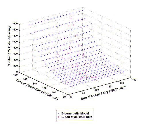
Figure 1. Number of surviving 3 year olds as a function of time of ocean entry and size of ocean entry.
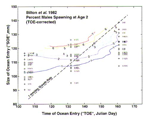
Figure 2. Percent of males returning at age 2 to spawn reflects growth characteristics, which are a function of time of ocean entry and size of ocean entry.
The data presented in Shapovalov and Taft (1954) are 8 years of measured SOE and TOE, as well as total returns (not identified by SOE, TOE) at ages 2 and 3 of naturally spawning fish. Our analyses of those data show: (1) that mortality rates estimated for each year from the fraction surviving to spawn at age 3 are significantly correlated with ocean temperature, and (2) our analysis of the effect of fish size is in progress.
GLOBEC NEP field studies will of necessity focus on the early ocean stage of salmon life history, yet in spite of the oft-stated belief that year class abundance is set at that stage, it is clear ocean conditions also influence CCS species in the year they return to spawn (Johnson 1988, Pearcy 1997). To understand the results of field studies, GLOBEC NEP needs to know the answer to the question: How does the combination of environmental variability in the juvenile stage and the adult stage affect population abundance? To answer this question, we examined behavior of an age-structured model that was essentially a Leslie matrix with reproduction determined by a Beverton-Holt stock-recruitment relationship. The age structured part of the model is of the form
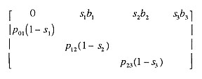 where pmn is the fraction surviving from age m to n, sn is the fraction spawning at age n, bn is the fecundity at age n, and recruitment each year is determined from a Beverton-Holt function of the product of the first row and the age vector. Our analyses (Figure 3) indicated: (1) random variability in p01 and p23 had the same effect on population abundance, and (2) simultaneous variability in both had an additive effect on the logarithm of abundance. Correlation between the two generally increased their effect, except in the case of obligate semelparous populations. These results indicate that if the ocean environment has the same effect on both juvenile and adult stages (e.g., ENSO or upwelling affecting overall productivity of prey for both stages), for chinook salmon species, the consequences will be greater than if it affected each independently, while for coho salmon (for which females are obligate semelparous), the population consequences will not depend on whether the mechanisms are the same.
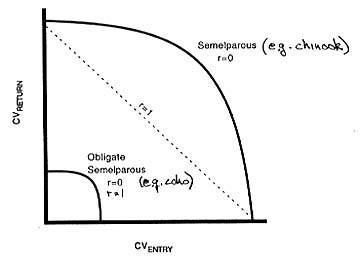
Figure 3. Results: (1) Effects are greater on obligate semelparous species (e.g., coho). (2) Effects on log abundance are additive if uncorrelated (r=0). (3) If the effects are correlated (r=1), abundance is less (probability of extinction is higher) for combinations of effects IF population is not obligate semelparous (e.g., chinook), but are unaffected IF obligate semelparous (e.g, coho).
In a third population level study, we investigated the way in which California Current salmon populations would be expected to respond to environmental variability on two dominant time scales, 5-10 year and multi-decadal (cf., Steele and Henderson 1984). The results (Figures below) showed how a semelparous species with a Beverton-Holt stock/recruitment relationship (as seen in coho salmon stocks) followed slowly varying periods of high and low ocean survival, but have qualitatively different behavior (more vulnerable to extinction) at low ocean survival, and also (unexpectedly) how extinction probability increases with increasing period of decadal scale variability.
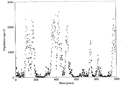
Figure 4. As the ocean environment of an obligate semelparous population (e.g., coho) shifted between high and low survival (at times corresponding to a Poisson process with mean of 15 years), the population was not merely high when survival was high and low when survival was low, but rather spent much more time at low abundances.
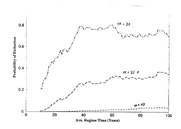
Figure 5. And the probability of extinction increased with the period of the cycles between favorable and unfavorable survival.