
Report of
RVIB Nathaniel B. Palmer Cruise 0204
to the
Western Antarctic Peninsula
31 July to 18 September, 2002
This report was prepared by Peter Wiebe, Eileen Hofmann, Bob Beardsley, Chris MacKay, Kendra Daly, Jose Torres, Scott Gallager, Christine Ribic, Erik Chapman, Ryan Dorland, Frank Stewart, Jenny Boc, Gareth Lawson, Yulia Serebrennikova, Gustavo Thompson, and Francisco “Chico” Viddi with assistance from colleagues in the scientific party, and of the Raytheon Support Services. Dicky Allison provided assistance in proofing the text. This cruise was sponsored by the Office of Polar Programs at the National Science Foundation.
United States Southern Ocean
Global Ocean Ecosystems Dynamics Program
Report Number 8
Available from
U.S. Southern Ocean GLOBEC Planning Office
Center for Coastal Physical Oceanography
Crittenton Hall
Old Dominion University
Norfolk, VA 23529
Acknowledgments
This was the fourth and final broad-scale survey cruise to the Southern Ocean GLOBEC Study site on the Western Antarctic Peninsula. In spite of very formidable pack ice conditions in much of the area, the N.B. Palmer was able to take us to much of the area in which we wished to work and we were able to accomplish much of the science that we set out to do. This was due in part to the skill and expertise of Captain Joe and the officers in working in winter ice conditions. It was also due to the fine technical assistance we have received from all ten members of the Raytheon Marine Technical Support Group. The crew of the Palmer also played an important role in keeping the morale high. A special thanks to Ernest Skelly and his galley crew for their culinary expertise. The success of the cruise was due to the collective efforts of all of these individuals. Throughout the cruise there was a camaraderie and friendliness among all the participants that made this expedition a great pleasure.
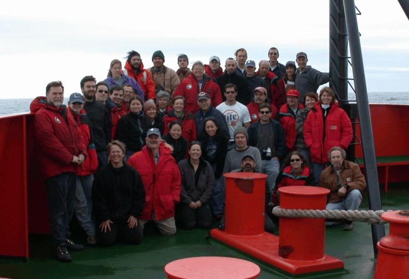
NBP0204 Cruise Participants on the RVIB N.B. Palmer
Kneeling Row1 (L-R):Dicky Allison, Scott Gallager, Nancy Ford, Phil Alatalo, Jamee Johnson, Jose Torres
Crouching Row2 (L-R): Jenny Boc, Emily Yam, Alec Scott
Row 3 (starting left of middle): Eileen Hofmann, Karie Sines, Susan Beardsley, Chris Ribic, Chris Shepherd, Todd Johnson, Tom Bailey (back), Ryan Dorland (front), Chris MacKay, Yulia Serebrennikova, Kendra Daly.
Row 4: Peter Wiebe, Sarah Dizick, Gareth Lawson, Frank Stewart, Gustavo Thompson, Bob Beardsley, Melanie Parker, Chico Viddi, Erik Chapman, Baris Salihoglu, Kathleen Gavahan, Jason Zimmerman, Fred Stuart, Frank Welte, Partricia Jackson, Steve Bell, Joe Donnelly, Kerri Scolardi, Stian Alesandrini.
TABLE OF CONTENTS
1.0 Hydrography, and Circulation
1.2 Data Collection and Methods
1.2.1.1 CTD Salinity Calibration
1.3.2 Water Mass and Circulation Distribution
1.4 Hydrography/Circulation Highlights from all SO GLOBEC Cruises
2.0 Microstructure Measurements with CMiPS
2.2 Instrumentation and Data Collection
3.0 Meteorological Measurements
3.3 Data Acquisition and Processing
3.4 Description of Cruise Weather
3.5 Description of Surface Fluxes
4.4 Preliminary Results for Nutrient Concentrations
6.1 Zooplankton Sampling with the 1-m MOCNESS Net System
6.2.1 Acoustics Data Collection, Processing, and Results
6.2.2.2.3 Video Recording and Processing
6.2.2.2.4 Plankton Abundance and Environmental Data
6.2.2.3 VPR Preliminary Results
6.2.3 Water column hydrographic and environmental characteristics
6.3 ROV observations of larval krill
6.3.2 Description of individual deployments
6.4 Microplankton Distribution, Abundance, and Swimming Behavior
6.5 Ingestion and Clearance of Microplankton and Particulates by Krill Furcilia
6.5.2.1 Experiment 1, 25 Aug 2002
6.5.2.2 Experiment 2, 30 August 2002
6.5.2.3 Experiment 3, 30 August 2002
6.5.2.4 Experiment 4, 01 September 2002
6.5.2.5 Experiment 5, 03 September 2002
6.5.2.6 Experiment 6, 06 September 2002
6.5.2.7 Experiment 7, 08 September 2002
6.5.2.8 Experiment 8, 10 September 2002
6.5.2.9 Experiment 9, 12 September 2002
6.5.2.10 Experiment 10, 13 September 2002
6.6 Operation and use of the Simrad EK500
7.0 Optical Plankton Counter and ADCP Studies of Zooplankton
8.0 Seabird and Crabeater Seal Distribution in the Marguerite Bay Area
8.2 Methods, Data Collected, and Preliminary Results
8.3.4.3 Snow Petrel (Pagodroma nivea)
8.3.4 4 Antarctic Petrel (Thalassoica antarctica)
8.3.4.5 Adelie Penguin (Pygoscelis adeliae)
8.3.4.6. Emperor Penguin (Aptenodytes forsteri)
8.3.4.7 Crabeater Seal (Lobodon carcinophagus)
9.0 International Whaling Commission Cetacean Visual Survey
9.4 Preliminary Findings/Discussion
10.0 Krill Distribution, Physiology and Predations
10.4.1 Abundance and Distribution
10.4.3 Physiological Measurements
11.0 Fish and krill ecology/ krill physiology
11.2.1 Fish and large krill (micronekton) abundance
11.2.2 Under-ice abundance of krill larvae
11.2.3 Respiration and excretion measurements
11.3.1 Fish and large krill (micronekton) abundance
11.3.2 Under-ice abundance of krill larvae
11.3.3 Respiration and excretion measurements
12.0 Distribution, Abundance, and Activity of Sea Ice Microbial Communities
12.3 Preliminary results/observations
APPENDIX 2. Summary of the CTD casts
APPENDIX 3. Summary of the water properties
APPENDIX 4. Summary of the XBT casts
APPENDIX 5. Summary of the XCTD casts
APPENDIX 6. NBP0204 CMiPS Data Summary
APPENDIX 7. Ctenophores removed from 1-m MOCNESS tows
APPENDIX 8. BIOMAPER-II Deployment Log
APPENDIX 9. Microzooplankton sample log.
APPENDIX 10. Simrad acoustics data log
APPENDIX 11. Fish and krill caught in 10-m MOCNESS Trawls on NBP0204
APPENDIX 12. Log of ice stations
The U.S. Southern Ocean GLOBEC Program is in its second and last field year. The focus of this study is on the biology and physics of a region of the continental shelf to the west of the Western Antarctic Peninsula extending from the northern tip of Adelaide Island to the southern portion of Alexander Island and including Marguerite Bay. The primary goals are:
1) To elucidate shelf circulation processes and their effect on sea ice formation and Antarctic krill (Euphausia superba) distribution.
2) To examine the factors that govern krill survivorship and availability to higher trophic levels, including seals, penguins, and whales.
In the second year, the field program began with a mooring cruise in February aboard the R/V L.M. Gould during which a series of water column moorings and a series of bottom mounted moorings (to record marine mammal calls and sounds) were recovered from the first year of deployment across the continental shelf off Adelaide Island and across the mouth of Marguerite Bay. A sub-set of the moorings was replaced for the year two observations. A pair of cruises took place during April and May of 2002. A process cruise took place on the R/V L.M. Gould and the third in the series of four broad-scale cruises took place aboard the RVIB N.B. Palmer. This report describes and details the fourth and last broad-scale cruise to take place this year. As with the past three cruises, this was a joint ship operation with the R/V L.M. Gould, which conducted process studies in the same geographic region. Our effort was mainly devoted to developing a shelf-wide context for the process work conducted aboard the R/V L.M. Gould and for the modelers who will be using both the broad-scale and the process data in their model computations. Our specific objectives with regard to the broad-scale survey were:
1) To conduct a broad-scale survey of the SO GLOBEC Study Site to determine the abundance and distribution of the target species, Euphausia superba and its associated flora and fauna.
2) To conduct a hydrographic survey of the region.
3) To collect chlorophyll data, nutrient data, and to make primary production measurements to characterize the primary production of the region.
4) To collect zooplankton samples with a MOCNESS at selected locations throughout the broad-scale sampling area.
5) To survey the seabirds throughout the broad-scale sampling area and determine their feeding patterns.
6) To survey the marine mammals throughout the broad-scale sampling area both by visual sightings and by passive listening techniques.
7) To map the bank-wide velocity field using an Acoustic Doppler Current Profiler (ADCP).
8) To collect acoustic, video, and environmental data along the tracklines between stations using a suite of sensors mounted in a towed body (BIOMAPER-II).
9) To survey the under-ice distribution and abundance of krill larvae using an ROV equipped with a VPR, ADCP, and CTD.
10) To collect meteorological data.
In addition, two process-oriented groups were present on this cruise whose primary objectives were:
1) To determine the abundance and distribution of micro-nektonic krill predators, primarily fishes within the study area.
2) To determine rates of metabolism and excretion of all life stages of krill.
3) To assess numerical abundances of krill larvae underneath sea ice using SCUBA and videography.
4) To capture krill larvae underneath sea ice using SCUBA and hand nets for experimental manipulation.
5) To take samples of the surface layer under the ice to assess food concentrations.
6) To freeze all life stages krill to assess composition, and biochemical indicators of condition.
7) To evaluate the behavioral and physiological overwintering strategies used by different life history stages of the Antarctic krill, Euphausia superba.
8) To assess the sexual maturity stages of female krill during winter in relation to environmental parameters.
The Southern Ocean GLOBEC grid on this cruise was composed of 85 station locations distributed along thirteen lines perpendicular to the coast (Figures 1, 2). Line 1 lay at the northern end of Adelaide Island and line 13 lay offshore of Charcot Island some 500 kilometers southwest of line 1. The center of the grid included Marguerite Bay. Because pack ice usually covers the entire grid area during the winter period, a ship like the RVIB N.B. Palmer with ice breaking capability was needed to get to the stations. In fact, some of the pack ice was so thick and formidable, that even the Palmer could not get to some of the stations during the winter cruise. Our companion ship, the R/V L.M. Gould, had an ice strengthened hull, but lacked the kind of ice breaking capability needed to move through most of the pack ice in the area. The Gould, however, was able to move through most of the ice pack if following the Palmer. Instead of starting in the northern sector and working our way to the south as had been done on the previous three survey cruises, the fact that we were providing assistance to the Gould so that it could work in pack ice beyond its capability meant a different approach had to be taken. Thus, the strategy for this cruise was to divide the grid into four sectors: southern (stations 65 to 85), central (stations on lines 5 to 8 not including those in Marguerite Bay), Marguerite Bay, and northern (stations 1 to 23). Approximately 7 to 10 days were allocated for work in each sector with time in between for the two ships to convoy to the next sector while conducting penguin and marine mammal work along the way. While the L.M. Gould was situated in a central location at a process station in a given sector conducting time-series studies of ice structure and dynamics and marine predator work, the N.B. Palmer surveyed the sector. We were able to work in the three sectors along the continental shelf, but the pack ice in Marguerite Bay proved too challenging to move into and that area was not sampled.
Prior to the start of the work on the grid, both ships met in Crystal Sound, the embayment just north of Adelaide Island, for a transfer of equipment and supplies and three days of joint science operations. This provided the investigators on the Palmer their first opportunity to deploy the over-the-side equipment and to begin collecting krill and other species for experimental work.
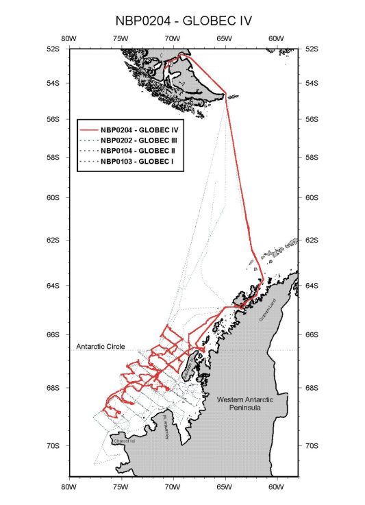 Figure 1. RVIB Nathaniel B. Palmer (NBP0204) cruise track (solid red line) and
cruise tracks from the previous three Southern Ocean GLOBEC broad-scale surveys.
Figure prepared by Kathleen Gavahan.
Figure 1. RVIB Nathaniel B. Palmer (NBP0204) cruise track (solid red line) and
cruise tracks from the previous three Southern Ocean GLOBEC broad-scale surveys.
Figure prepared by Kathleen Gavahan.
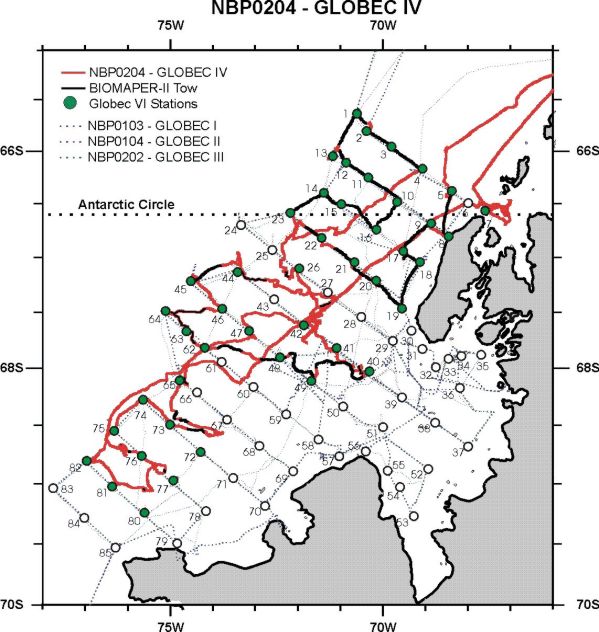 Figure 2. The Southern Ocean GLOBEC broad-scale survey grid and trackline, showing
locations of stations and some along-track observations. Locations of specific activities are in
the individual reports and in the event log (Appendix 1). Previous broad-scale cruise tracklines
are indicated as dashed lines. Figure prepared by Kathleen Gavahan.
Figure 2. The Southern Ocean GLOBEC broad-scale survey grid and trackline, showing
locations of stations and some along-track observations. Locations of specific activities are in
the individual reports and in the event log (Appendix 1). Previous broad-scale cruise tracklines
are indicated as dashed lines. Figure prepared by Kathleen Gavahan.The Crystal Sound area has on past cruises been a “hot” spot for krill and their associated predators (seals, penguins, seabirds, etc), and a part of the work involved a study of the hydrographic setting to provide some insight into why this is so.
The work on the grid was a combination of station and underway activities (See the Event Log, Appendix 1). The along-track data were collected from the Bio-Optical Multifrequency Acoustical and Physical Environmental Recorder (BIOMAPER-II), the ADCP, the meteorological sensors, and through-hull sea surface sensors, XBTs, XCTDs. At the stations, a CTD/Rosette equipped with oxygen, transmissometer, and fluorometer sensors was cast to the bottom. In water depths less than or equal to 500 m, a Fast Repetition Response Fluorometer (FRRF) was added to the Rosette. At selected stations, a 1-m and a 10-m Multiple Opening/Closing Net and Environmental Sensing System (MOCNESS) were towed obliquely between the surface and near the bottom or 1000 m if the bottom was deeper for collection of zooplankton (335 μm mesh) and micronekton (3 mm mesh). A Tucker Trawl was used to make collections of live animals for use in shipboard experimental studies. A pair of 1-m ring nets were used in tandem off the stern of the Palmer to collect live zooplankton, principally furcilia of Euphausia superba from the upper 10 m of the water column. A 1-m ring net tow was also used to make a mixed-layer collection of zooplankton at some stations. The failure of the new Simrad multi-beam system to perform satisfactorily during sea trials prevented its use to acquire bathymetric data on this cruise.
31 July to 1 August: The cruise got underway at 1400 on 31 July when we left the port of Punta Arenas, Chile after a week of intense setup of the equipment and laboratory spaces needed for the work at sea. The setup and testing of gear went very smoothly as a result of the superb planning and assistance rendered by the Raytheon Technical Support Group. Although the air temperature was right around freezing, skies were partly cloudy, and wind and sea conditions were calm. Thus, it was a smooth start to the cruise.
Shortly after leaving port, we had our first ship orientation and safety meeting with Chief Mate Mike Watson. An integral part of the first meeting on a cruise is the putting on of a survival suit, which is issued to each person, and the exercise of getting the entire science party into a large life boat and strapped in, this time with our survival suits on. The safety meeting was followed by brief orientation comments from Marine Project Coordinator Chris Shepard and Chief Scientist Peter Wiebe. Then there was a deck safety briefing led by Stian Alasandrini and an Information Technology orientation [email, networking, computer support in general] led by Paul Huckins. Shortly after dinner while in the embayment between the two narrows in the eastern portion of the Straits of Magellan, a deployment of BIOMAPER-II was done to allow the marine Technicians and others who would be handling the system get some practice with launch and recovery under good sea conditions. It was also done to test the electronics and sensor systems on the towed body, and to adjust the tail elevator to minimize variation of pitch and roll from horizontal under normal towing conditions. Around 2030 at the pilot drop-off point on the eastern end of the Straits of Magellan, three individuals (Peter Martin of Raytheon, and Terry Hammar and Andy Girard, both from WHOI) who were assisting in the port setup of the hardware and software associated with BIOMAPER-II and the ROV, left the ship along with the pilot.
The course to the survey area again took us down the eastern side of the tip of South America (Argentina), through the Estrecho de La Maire, and out into the Drake Passage. Because of the extensive ice pack coverage of the survey area and areas substantially to the north and because of the need to closely coordinate our trackline with that of the L.M. Gould, which is dependent upon the Palmer for ice breaking services, we would be steaming a line that would take us into the inside passage (Gerlache and Bismark straits) and then down to Crystal Sound. Crystal Sound is just north of Adelaide Island and at the northern end of the survey grid and it will be the first site for joint ship operations. The distance from Punta Arenas to Crystal Sound is approximately 1100 nm.
During 1 August, we steamed along the southern Argentina coast in calm seas and light to moderate winds (<20kts). Skies remained overcast and the barometric pressure dropped slowly from around 1006 mb in the morning to 996 mb in the late evening. Air temperatures were around 5 C. Taking advantage of the nice sailing weather during the afternoon, a science meeting was held to discuss in more detail the station work plans and also to provide some of the investigators (Bob Beardsley, Eileen Hofmann, Chris MacKay, Erik Chapman, Kendra Daly, and Scott Gallager) with an opportunity to describe findings from previous cruises as a context for work that will occur on this one. The meeting ended with the Palmer just entering Estrecho de La Maire in the last light of the day. Snow-capped peaks of the mountains of Isla de los Estados to the east and those on Peninsula Mitre on the mainland to the west were silhouetted against a darkening sky.
2/3 August 2002: The Drake Passage is a dreaded stretch of water extending down below the southern tip of south America to the continental shelf region of the Western Antarctic Peninsula. High winds and high seas are frequently present and on the Southern Ocean GLOBEC cruises the investigators have had to steel themselves for a very uncomfortable ride across the Passage to get to the study site off Marguerite Bay. On the Austral fall cruise this year, the Passage lived up to its reputation, and only a few hardy souls were up and around during the first days of the transit. On this cruise, we were spared the fury of its storms and made it across with moderate winds and seas during an interlude in the winter storms. That is not to say that all was well. The seas were still rough enough to make a number of individuals feel seasick.
Much of 2 August was spent steaming within the 200 mile Argentine economic zone. Argentina has severe restrictions on the scientific information that can be recorded by foreign ships such as the N.B. Palmer. Thus, most electronic sensors acquiring data by electronic means were turned off. By special arrangement, the Acoustic Doppler Current Profiler (ADCP) data were being logged as were the navigation data needed to interpret the current meter data. Also, incidental observations were made of seabirds and mammals. Once the 200 mile limit was reached (around 1630), Expendable Bathythermograph (XBT) observations commenced and the along-track sensing system for recording sea surface temperature, salinity, fluorescence, PCO2, bottom depth, and meteorological data began recording data. For a number of groups, the days steaming were used to complete the setups of their laboratory space and experimental equipment, and to rig the equipment to be deployed in the ocean.
During the morning of 2 August, the winds were in the 15 to 25 kt range out of the west. Around 0800 at -57 18.83S; -64 14.73W, we crossed a front (possibly related to the Subantarctic Front) and in a matter of minutes the sea surface temperature went from 2.2 C to -0.63 C. There was a similar shift in the air temperature, although not as abrupt. The skies were partly cloudy throughout the day and the sea was ice free, although the first iceberg of the cruise was spotted during the day. In the evening, there were light rain showers. Around midnight as we were approaching 60 S, we encountered the northern edge of the pack ice in the form of isolated patches of sea ice. This position was much further north than where we encountered it last year at this same time of year. In the morning of 3 August, overcast skies in the Passage again gave way to a mixture of sun and clouds. Bright sun highlighted the white pack ice and the numerous moderate-sized icebergs that we steamed past on our way to the Boyd Strait - our entrance between Snow and Smith Islands into the inner passageway leading to the south along the Gerlache and Bismark straits. The winds stayed out of the west below 25 kts, but during the day it was cold on deck with the air temperature around -2C. In the late afternoon, snow squalls enveloped the Palmer and the ship’s speed had to be reduced for a time because of the poor visibility.
4 August 2002: The long transit from Punta Arenas, Chile to the first work site in Crystal Sound was nearly over by the end of 4 August. During the night, the N.B. Palmer steamed along the Bransfield Strait and into the northern end of the Gerlache Strait, while the physical oceanography group continued the XBT survey of the area. A sliver of a waning moon was setting in the northwest just as the first light of dawn, which took place around 0800, allowed the mountain ranges on both sides of the strait to become visible. For the most part, the transit was ice free allowing the ship to maintain a normal cruising speed of 10 to 11 kts.
The morning was an extraordinary opportunity to see the inner passageway (Gerlache Strait) in all its splendor. Clear skies for most of the morning provided superb views of the snow-covered peaks and mountain glaciers that were sparkling in the bright sunlight. Broken gray clouds were draped over some of the peaks adding an extra dimension of texture to an already wondrous scene. Although the sun was out, winds of around 25 kts out of the west kept the wind chill well down into minus numbers and for the many in the scientific party taking pictures, being out on deck was a bit brutal.
The weather in this part of the world is also extraordinary in that it changes rather rapidly. Early in the morning the air temperature was around -1.9 C and the sea temperature was -1.268. The barometer remained fairly high at 1006.1 mb. By early afternoon, low clouds moved in and the mountain peaks were obscured. As we moved westward along the Bismark Strait in the late afternoon (1800) toward the open water of the Western Antarctic Continental Shelf, the barometric pressure, which had begun to climb earlier in the day, reached a remarkable 1017 mb, while the air temperature dropped to -8.6 C and the winds dropped to less than 5 kts.
Around 1830, we made the turn to head south towards the entrance to Crystal Sound. Water temperatures of -1.764 C (approaching the freezing point), were substantially colder than in the inner passage. Within an hour of making the turn, we ran out of open water and were back into the pack ice and the consequent slower ship’s speeds (6 to 7 kts)
5 August 2002: According to the “Geographic Names of the Antarctic”, Crystal Sound was so named relatively recently in 1960 “...because many features in the sound are named for men who have undertaken research on the structure of ice crystals.” It is an apt name also because ice dominates the seascape in the area now. Our transit to the Sound ended about 1230 on 5 August at a station south of Watkins Island (-66 31.37S; -67 16.15W). In contrast to yesterday, which started off bright and sunny, dark clouds hung low most of the day blending in with the pack ice so that the horizon was often not visible. Although the Palmer moved easily on two engines through the pack ice for a good portion of the steam down to the Matha Strait entrance to Crystal Sound, as we made the approach to the strait, the ice pack thickened significantly and the power of four engines was needed to get us into the sound and to our first working location. During the late evening of 4 August while steaming southwest out along the outer margin of the series of Islands leading to the study site, radio communications with the L.M. Gould revealed that they were steaming into Pendleton Strait and would head south to the east of Lavoisier Island down to Crystal Sound rather than following along our trackline, which lay to the west of the Island. They thought that by taking that route, they had a better chance of encountering seals and penguins to work on, although a number of sightings were made from the Palmer during the day.
First up in the science program for the two and a half day stay in the sound was a SCUBA dive under the ice to look for krill larvae and other zooplankton that live in close associated with the undersurface of the pack ice. The dive was done from a zodiac boat in a frozen lead opened up by the Palmer. The dive went well, although one of the diver handlers dressed for the cold, but not for in-water work, slipped getting down the ladder into the zodiac, and took a short plunge. Another person quickly got suited up and took the place in the boat, while the other, unhurt, dried out. Interestingly, no krill were observed during the dive. While the dive was underway, the first CTD cast was undertaken and went well. BIOMAPER-II was deployed for a calibration run off the stern of the Palmer after the divers returned, and the evening ended with the starting of a series of CTD casts in a transect line across the Matha Strait inlet to Crystal Sound.
The weather during 5 August was dark, dreary, and cold, although the wind stayed moderate (15-20 kts) to low (<10 kts) all day. The air temperature started out in the early morning hours at -9.4 C and the barometer reached a peak of 1019.2 mb. By evening, the air temperature had warmed some to -4.7 C; the barometer remained high (1018.6 mb). The sea water temperature was at the freezing mark (-1.824C).
6 August 2002: The sixth of August found us working for a second day in Crystal Sound. In the first light of the day, we could see that the L.M. Gould had made it to the work site using the back route to the sound and the investigators were now able to work in the area. Our effort during the night and early morning was spent doing a CTD section across the mouth of Matha Strait. At the end of the section, a joint ice collection and ROV under-ice survey was done. The Palmer then steamed to a site just south of the Barcroft Islands (-66 30S; -67 01W). Along the route, we passed within a quarter of a mile of the Gould and could see a group of investigators working on a crabeater seal that they had managed to sneak up on and anesthetize. They were making physiological and biochemical measurements and attaching a small tag equipped with sensors and a satellite telemetry system to the back of the seal’s head. At the Barcroft site, a calibration of an HTI acoustic system was undertaken during the latter portion of the morning. A search for Adelie penguins that were hauled-out on the ice after feeding was started around 1300 and within a short time 10 individuals were spotted on a large floe. The Palmer was able to move slowly up to the edge of the flow without the penguins leaving the area and a party of investigators were deployed onto the ice with the personnel carrier operated from the ship’s crane on the bow. Three of the penguins were captured and diet-sampled before being released. Late in the afternoon, the Tucker Trawl was used to make collections of live zooplankton, especially krill, for use in feeding, growth, and physiological experiments over the next few days. Two back-to-back tows were done near the entrance to Crystal Sound with the second tow catching substantial numbers of adult krill.
The early evening was spent steaming to a rendezvous point where an exchange of equipment and supplies took place between the Palmer and the Gould. The pack ice limited the drift of the vessels and made it possible to position the ships with the bow of the Palmer within a few meters of the stern of the Gould. The exchange was made using the bow crane on the Palmer to move cargo nets with the gear between the Palmer’s bow and the Gould’s stern deck. The transfers took about an hour, after which the Palmer steamed south to a location north of Laird Island (-66 41.8S; -67 08W) where a second CTD transect was begun to define the hydrographic characteristics of water flowing into Crystal Sound through Matha Strait.
In the morning before sunrise (0730), the skies were cloudy and the air temperature was -5.2 C. The barometric pressure (1017.4 mb) was down a bit from the last day or two and the wind was out of the south (177) at about 5 kts. The sea surface temperature was -1.795 and salinity was 33.845 psu. The morning turned beautiful with the sun breaking through the overcast skies so that there was a hazy cloudiness filtering the sunlight. In the mid-afternoon, there was a low thin foggy mist to the atmosphere and the sun, shining through, was a yellow ball with blurred edges. What little wind there had been in the morning died and it was calm throughout the afternoon and evening. During the transfer with the Gould, a very fine misty snow fell lightly and the air temperature was around -7 C.
7 August 2002: August 7 was our last day in Crystal Sound. In the wee hours, a CTD transect was run along the southern portion of the sound out to the entrance of Matha Strait. At the final CTD station location, a combined ice collection operation and an ROV under-ice survey were done. The Palmer then steamed back into Crystal Sound toward the location where the Tucker Trawl was done yesterday. The 1-m MOCNESS was accomplished successfully, but not without difficulty. The pressure sensor froze up during the extended setup time on the deck typical of a first tow and did not thaw out until about 20 minutes into the tow. On one occasion, the towing wire was caught by a large ice chunk that drifted into the wake and the ship had to stop and back up to free the cable. The same thing occurred later in the evening when the 10-m MOCNESS was towed for the first time on this cruise, but it did not affect the ultimate success of either tow. Both net systems had very nice catches in their respective nets, which showed a complicated vertical structure of the plankton and nekton living in the water column. The significant concentrations of krill in the Crystal Sound area at this time of year is likely a major reason why the many marine predators were present. We completed the work in Crystal sound in the late evening and then headed out Matha Strait to the west with the L.M. Gould close behind.
In general the work in Crystal Sound was quite successful. All of the instruments were deployed for the first time, and, with only a couple of exceptions, worked. The microstructure instrumentation had not yet worked when deployed on the CTD, but the trouble-shooting turned up several fixable problems and the system was operational when next put into the water. BIOMAPER-II suffered a failure of the transmitting circuitry for the 420 and 1000 kHz frequencies during the period of calibration two days earlier. Efforts to determine what component failed were not successful, but continued. The lower three frequencies remained operational and the system was survey-ready at the start of the grid work.
The benign weather pattern experienced over the past couple of days, dominated by a high pressure system, continued on 7 August. Although the air was cold - mostly between -8 and -10 C - the winds were light out of the southwest, so work on deck was comfortable. The barometer continued to fall slowly and varied from 1015 mb in the early morning to 1010 mb in the evening. Sea surface temperature remained at the freezing point (-1.845 C).
8 August 2002: Our first day on the transit to the southern sector of the Southern Ocean GLOBEC grid off Alexander and Charcot Islands was fraught with difficulty. After entering Crystal Sound on 5 August, there apparently had been a buildup of very dense brash ice just outside the entrance to the sound. Although we began the journey before midnight on 7 August, by mid-morning on the 8th, we had made about 6 nm and our progress was a snail’s pace. A part of the problem was that the wind was out of the northeast at about 20 kts and this had caused the ice to pack in close to the shore. While the Palmer could make it through this pack ice with relative ease, the L.M. Gould could not. Even with the Gould very close behind, the Palmer’s wake region closed up with the dense brash ice to such an extent that the Gould could not push forward through it and within a short time came to a stop. The Palmer then either had to back down to reopen the path in front of the Gould and start out again or to circle and come up alongside the Gould, cut right in front, and then move forward with the Gould again trying to follow behind. For most of the day the convoy went nowhere fast. About 1700, as we moved west beyond the vicinity of three very large icebergs, the character of the ice changed and the wake region no longer closed up so abruptly. The Gould finally could follow the Palmer and we were able to move consistently along the transit route to the southwest.
Several hours later while steaming off the northern end of Adelaide Island, the ice pack thinned significantly and there were pools of open water amongst the floes. An XBT survey with drops at 10 nm intervals was started in this area to see if the water column characteristics were indicative of offshore water coming into the area and contributing to an increased upward heat flux that reduced the rate of sea ice formation. Indeed, the deep water was much warmer, indicative of the ACC water coming onto the shelf.
The slow pace of the transit made it a good day to go computer virus hunting. The ship’s PC computers were hit by the klezH@mm virus making life miserable for many of the investigators and crew using PCs and causing significant problems with the data acquisition systems. The ship’s network was shut down in the morning and all of the laptop computers were brought to a main lab for virus checking and cleaning. All other PCs throughout the ship were also checked and cleaned. Virus checking had started a couple of days earlier when it first turned up, but a few computers were found to still have the virus. By late afternoon, all machines had been scanned/cleaned and the network brought back up with no sign of the virus.
During the day, the skies were overcast and, like a couple of days ago, there was almost no contrast between sea ice and sky. Huge icebergs, which dotted the area, blended into the background so that they were barely visible. The winds were persistently out of the northeast (050) around 20 kts. The air temperature varied from -2.5 C in the morning to -3.4 in the evening. The barometer continued its slow decline moving from 1006.2 mb to 1001.4 mb by evening.
9 August 2002: August 9 was a very different day from the 8th when we were stuck for a good portion of time and wondering if we were going to go anywhere. On the 9th, we were able to cruise along through the pack ice with no difficulty. Still we did not go very far because there were sufficient predators out on the ice to make the Marine Mammal and Bird Groups on the Gould want to stop and go to work. This was part of the plan for the steam to the southern section of the SO GLOBEC grid, so the investigators on the Palmer were ready with a series of tasks that could be undertaken quickly to take advantage of the break in steaming and kept working. The first encounter with penguins happened right after a fire and boat drill. The seabird observers were allowed to go back to the bridge after signing in and it was a good thing they did. Right at the end of the session in the Palmer’s level 3 conference room, the call came that a big group of Adelie penguins had been spotted. It was an exciting morning chasing penguins. A coordinated effort to capture some of them was mounted by both the Gould and the Palmer. Chris Ribic and Erik Chapman first spotted about 40 to 50 Adelies in a group on the ice pack ahead of the ship about 0930 hrs and they notified the Gould. Then the Gould moved ahead of the Palmer to get next to the penguins, but the penguins started moving away. So the Palmer moved up to cut the escape route and the penguins moved within a short distance of the Palmer before turning back towards the Gould. By this time about 10 investigators from the Gould had been put onto the ice using the forward crane and personnel basket. The investigators began to walk over the ice pack to the penguins. They stopped halfway to the Palmer, fanned out, and crouched down when they realized that the penguins were now moving right back to where they were. When the penguins were within feet of the investigators, the investigators sprang into action capturing with nets quite a number of the penguins. It was an amazing sight with the sun coming up in the background just behind the Gould, which from our vantage point, was directly in line with the investigators and the penguins. It was a scene right out of a movie. After the free-for-all, the Palmer was positioned to allow the HTI acoustic system and the CMiPs/CTD to be deployed as our first attempt at a rapid response to get some work done. Having both pieces of gear in the water turned out not to be good for Kendra Daly’s work with the HTI system. The ship had to keep the propellers going to keep the CMiPS/CTD area clear of ice and this messed up Kendra’s ability to keep a calibration ball under the pair of transducers.
The Gould had barely completed the work on the penguins when they spotted four crabeater seals on the ice nearby. So they again deployed a team on the ice, drugged one of the seals, and then did their physiological/biochemical measurements and satellite tagged it. The HTI system was again deployed for some more calibration work, but ice chunks kept drifting in and interfering, so the ship moved around and a nice hole was formed. In the end there was only about 45 minutes of measurements, which was not enough to complete the work.
Late in the day, the seal work was completed and we again started to move to the south, but only for a mile or two. Another set of penguins were seen and the Gould made a bee-line for them. On the third stop, Frank Stewart and Jenny Boc took a group on to the ice to do ice-coring and Scott Gallager did an ROV under-ice survey. Once the Gould finished their work, the work on the Palmer was stopped and the two ships again set off along a trackline headed for the southern sector of the grid at about 5 kts.
The weather on the 9th was ideal for the science activities on both ships because the winds were light (<10 kts) and there was a good bit of sun during the day, after the morning clouds gave way to clearer skies. The air temperature was warmer in the morning (-4.6 C at 0900) than in the evening (-9 C at 1900). The lower portions of the mountains of Adelaide Island to the east were clearly visible during the morning sunrise. By mid-afternoon, while the sky was still partly cloudy with a high thin overcast, the mountains of Adelaide Island were clearly visible in their entirety. The barometer continued to fall slowly from 991.9 mb in the morning to 986 mb in the evening. The pack ice continued to be 10/10 with infrequent leads.
10 August 2002: The third day (10 August) of the convoy transit by the N.B. Palmer and the L.M. Gould from Crystal Sound to the vicinity of Station 77 on the Southern Ocean GLOBEC grid mostly consisted of steaming. The marine mammal group on the Gould led by Dan Costa had decided to wait to tag and to make measurements on more seals until getting into the southern portion of the grid. This restraint occurred in spite of the fact that a substantial number of seals were present along the trackline. The penguin group led by Heidi Geisz on that vessel were only interested in sampling penguins hauled out on the ice pack in the afternoon after they had been feeding and none were seen. So we made good progress during the early part of the morning in ice pack that was easy to move through. The fast steaming through the ice pack came to an end about 1000, when the Palmer encountered substantially thicker ice pack that was a jumble of broken and rafted chunks of ice half a meter to a meter thick. Backing and ramming was required to make it forward. This was to some extent expected since we crossed the line marked by the southern outer portion of Marguerite Bay and the northern tip of Alexander Island and entered the southern sector of the grid. Last year, we were in substantially thicker ice once we got south of this line and this year it seems to be the same.
Just after noon the Gould called to express concern about the speed at which we were moving toward Station 77 and to raise the possibility that they take up residency to the east of our position at that time (approximately at station 60). A review of the most recent ice images revealed that the open ocean and ice edge had moved considerably east relative to where it was when we left Punta Arena, Chile at the end of July and now included portions of the SO GLOBEC grid. This was quite unexpected. Also areas to the south appeared in the image to have better ice conditions from a steaming point of view than what the convoy was plowing through at the time. The ensuing discussion resulted in their dropping the idea of going east and instead they worked with us to get to the original destination by heading offshore to the northwest toward the open water. The plan then was to turn to the southwest and head down the outer line of stations (65, 74, 75) before heading to the southeast along survey line 10 to station 77. This added considerable distance and time to the transit, but made it possible to get to the desired location. This plan was executed.
During the night of 9/10 August, the air temperature dropped to -10 C, warmed during the day to around -6.4 C, and then dropped back down in the evening to -9.0 C. Winds were light at about 7-8 kts out of the north (349) in the morning, shifted to about 8 kts out of the southwest (223) by mid-afternoon, and were stronger in the evening, 20-22 kts out of the southwest (233). This change was reflected in the barometric pressure that was at 979.9 mb in the morning, 977.8 mb in mid-afternoon, but 981.0 mb and rising in the evening. The skies were mostly cloudy during the day, but quite variable. In the morning, it was very cloudy with the sea ice merging seamlessly with the gray sky so that the horizon was not discernable. There were some snow flurries and light freezing rain. Then it cleared some and off in the distance there were patches of blue sky. On occasion the sun was like a spotlight shining on icebergs in the distance turning them to a brilliant white against a dark background. Beautiful!
11 August 2002: The N.B. Palmer and the L.M. Gould completed the convoy to the southern sector of the SO GLOBEC grid on 11 August. The strategy of moving out to the continental shelf area to avoid the heavy ice pack worked well. By mid-morning on 11 August, we were just 8 nm from Station 76 and had steamed into much harder pack ice when the Gould called with a request that we stop and return to a position about 3 to 5 nm back on the trackline. About 1230, we arrived at the location (-68 41.254S; -76 11.348W) chosen by the Gould for their first week-long process study site. There was lot of activity in the afternoon getting the Gould into place. A transfer of some samples to be used to inter-calibrate instrument systems on both ships as well as some other equipment took place shortly after the Gould had deployed their gangway onto an ice floe. Three investigators from the Gould walked several hundred meters across the pack ice to the Palmer and came aboard on the personnel carrier. The three stayed for about 30 to 40 minutes before trekking back to the Gould. The Palmer then made a large pond in the pack ice some distance away from the Gould in order to deploy the CTD for a cast to characterize the hydrography of the site. This cast was done by the Palmer instead of the Gould so that they did not have to cut a hole in the ice outside their Baltic Room CTD hanger door immediately. BIOMAPER-II was deployed in that same pond to make additional calibration measurements.
Finally, we got underway for the start of the grid survey about 2030. As the Palmer left the Gould’s work site and started back along the trackline toward station 76, we took advantage of a large lead created by the passage of the ships earlier in the day to do a 10-m MOCNESS tow followed by a live animal collection with the Tucker Trawl, which ended just after midnight.
During the day, a number of marine mammals paid us a visit. A seal climbed up on to the ice pack shortly after the Palmer “parked” at the Gould work site in the early afternoon and then slid back in and disappeared. Minke whales were seen in the wake areas of both ships in the afternoon and during the steam in the morning an Orca was also seen. During the BIOMAPER-II calibration, five Crabeater seals came swimming into the open water area where it was about to be deployed. They thrashed and frolicked around and came up and snorted at us peering down on them from the fantail.
The weather as usual was quite variable. In the late night (0045), the air temperature was -15 C and the barometer was 982.9 mb and rising as a low pressure system passed through. Winds were out of the west about 10-15 kts. Around 0700, the temperature has dropped to -19.2 C, the barometric pressure was a bit higher (985.5 mb), and the winds were about the same. At sunrise, around 1000, skies were overcast with the only clear sky at the horizon. The sunrise was spectacular with brilliant reds and oranges giving swirls in the clouds a scorched look. At mid-day, the skies cleared out completely and the sun rose to 3 to 4 fingers (at arms length) above the horizon at high noon. The sun was brilliant reflecting off the snow and ice at that angle. We were treated again to a stunning sunset. After the sun had set, a red afterglow remained on the horizon and a new moon topped by a brilliant Jupiter hung above the Gould, which was off in the distance with its deck lights blazing. In the late evening, the air temperature was around -16 C, the barometric pressure continued to increase (994.1 mb), and the winds died down to 5-10 kts out of the west (249).
12 August 2002: This southern sector of the grid had the oldest and thickest pack ice in the survey area and proved very difficult to move around in. On 12 August, we steamed to station 76, the first grid station to be sampled on the grid after leaving the Gould late in the evening of 11 August. After work with the 10-m MOCNESS and the Tucker Trawl was completed while en route, BIOMAPER-II was deployed about 0100. Only about 40 minutes later, it had to be retrieved when the ridging in the ice pack proved too tough for continuous forward movement and Palmer had to resort to backing and ramming frequently. Two back-to-back CTD casts were made at Station 76 and then the steaming began for Station 77 near the center of the continental shelf. Around 1000, we came into an area of open pools of water and fairly large and smooth floes that were about ½ meter thick. The radar seemed to show more of the same ahead so we decided to deploy BIOMAPER-II. About the time we were ready to do the launch, a rubble field with substantial ridging was encountered that quickly brought the ship to a stop and also any idea of towyoing BIOMAPER-II. We never made it to the intended location of Station 77 because the ice pack was too tough to get through. Time constraints forced us to stop short and the station work was done in a large lead. Work completed included an under-ice dive, two CTD casts, an ROV under-ice survey, ice collection, and a 1-m MOCNESS tow. Because of the ice pack conditions, a decision was made to drop stations 78 and 79, stations located closer to shore. Late in the evening, we set off for Station 80 to the southwest instead.
The temperature moderated noticeably by mid-day on 12 August rising from around -20 C about 0100 to -2.2 C at 1300 as the barometric pressure dipped slightly from 995 to 987 mb. As the barometric pressure rose in the evening back up to 996 mb, the temperature dropped to -9.6 C. Winds were a moderate 12 to 15 kts out of the WNW (303) in the early morning, shifted directions to west later in the morning, and picked up to 21 to 27 kts by early evening. It snowed over-night leaving about ½ inch on the deck and in the morning there was a high overcast cloud layer and not much light from the sun. The contrast was very low making it difficult for the bridge to pick a course through the rubble and ridging in the ice pack to get to good floes. Periodically, a fog lowered visibility to only a few hundred meters.
13 August 2002: The pack ice in the southern sector of the SO GLOBEC grid proved to be a tough obstacle to overcome. In the evening of 12 August, we finished up work at station 77 around 2230 and headed for station 80 some 26 miles away. At 0730 on 13 August, we were still about 12 miles away and it was clear that we could not spend additional time trying to get there. A mile long lead was in the area and that is where the work intended for station 80 was done. The work in the lead included a CTD cast, a BIOMAPER-II time-series profile, and two Tucker Trawls to collect live animals for experimental purposes. About noon, the Palmer headed northwest toward station 81. We arrived at the station around 1615 after getting a break in the ice pack and making good time toward the end of the run. The station was done in another lead only 0.5 miles from the intended station location. After the CTD, a Tucker Trawl taken to get additional live animals to work with and, unlike the one taken earlier in the day, the catch was a good one. This was followed by a 1-m ring net tow in the upper 50 m. Around 1900, we again started steaming - this time for station 82 on the edge of the continental shelf.
A false fire alarm sounded about 2245 that turned into an unplanned drill. Everyone in the science party got to the level 3 assembly point very quickly. Apparently, the alarm was triggered by a smoke detector in the hydro lab where the nutrient auto-analyzer was located, but there was no smoke or fire.
In the wee hours of 13/14 August, a decision point was reached. The struggle to steam and work on survey lines 11 and 12 gave rise to the likelihood that as much or more survey time would be required to get to stations 83, 84, and 85 as was required to get to the earlier stations. This would jeopardize the possibility that we could cover the ten stations on survey lines 9 and 10 in the time remaining to work in the southern sector. Although some of those stations were likely to be unapproachable as well, the decision was made to drop the work on line 13 and instead head along the continental shelf toward stations 75 and 74 once the work was completed at station 82. This enabled us to focus our effort during the next 4 or 5 days on lines 9 and 10.
August 14 was cloudy with snow off and on throughout the day. The morning started out cold (-9.6 C at 0038), but warmed during the day and into the evening to -2.0 C by 2030. The barometer fell from around 995 mb in the morning to 984.8 mb at night. The winds were almost a repeat of the cycle on the previous day. They were light (~6 kts) out of the north around 0700, but changed to westerly by 1100 and picked up to around 20 kts and remained that way for most of the rest of the day. Around midnight, winds increased substantially and the air temperature dropped to -10 C, a portent of more extreme weather on 14 August.
14 August 2002: The biological and physical work in the southern sector of the SO GLOBEC grid continued for a fourth day aboard the N.B. Palmer. It was a day that was particularly clear and brutally cold. Gale force winds in the 30 to 40 kt range and -16 C temperatures made work on deck miserable. The pack ice continued to be very tough to move through in some places and more easily traversed in others, especially where there were leads. The steaming between stations, nominally 20 nm apart, could take six or more hours. It was a eight hour struggle to get from station 81 to station 82, located on the outer continental shelf. In the late night of 13/14 August, in spite of the high winds, a 1-m MOCNESS tow was completed in a lead. This was followed by an ROV under-ice survey and an abbreviated ice collection station. The high winds blew freshly fallen snow up into the air causing near white-out conditions and forcing the pack ice sampling to be stopped after a short period. Pack ice drift of about a knot under the sustained winds brought us closer to Station 75 and helped shorten the steaming time there. In the early afternoon, a pair of CTD casts, one for micro-structure measurements and the other for more general water column properties, and a live animal collection with the Tucker Trawl were completed there. Better ice conditions and continued pack ice drift allowed passage to station 74 further north along the outer shelf to be completed in about five hours. There another pair of CTD casts and a Tucker Trawl were completed in the late evening. The Tucker Trawl was done instead of a 10-m MOCNESS tow because the pack ice conditions for towing were judged to be marginal. Indeed, mid-way through the trawl, the towing cable was snagged by ice moving into the stern wake and before the ship could be stopped, the wire was strung out over the ice in the wake area some 50 to 100 m behind the ship. It took some time to clear the ice and bring the cable close enough to the stern to allow the net to be retrieved. Nevertheless, the catch provided planktonic animals for use in experimental studies on board the Palmer.
The weather provided both good and bad working conditions depending upon the scientific activity. For the seabird and marine mammal observers the clear skies and excellent visibility most of the day provided ideal viewing. The extreme cold made work on the deck difficult for everyone. The primary production incubators located on the helicopter deck proved particularly troublesome. The low temperatures caused pipes to break and seawater to flood a portion of the area late in the night. The MTs worked long hours to fix the incubators and to clear the area of slush and ice. Their efforts were very much appreciated.
The high winds first began about midnight on 13/14 August coinciding with a rapid drop in air temperature from around -2 C to -10 C. Winds out of the west southwest built rapidly into the 30 to 40 knot range and remained that strong for much of the day. The temperature dropped further and by 0732 was -16 C. It remained there until late in the evening when it dropped down to -19.2 C. By that time, the winds had subsided to the 8 to 12 kt range out of the southwest. The barometer stayed around 985 mb for a good portion of the day and only began to rise in the early evening reaching 994.3 mb by midnight. In spite of the cold and wind, it was bright and sunny. Before sunrise the first vestiges of day were evident on the horizon to the north as faint reds on a band of clouds. Overhead skies were dark and clear and stars were shining. The sun came up at 0945 as a bright orange ball that one could look at directely because of the filtering of the thin clouds on the horizon. The sky was clear for the most part and visibility was excellent. Large icebergs dotted the scene from morning to evening. There were also a number of long thin leads, which the Palmer used as passageways, and in which there were a number of seals and a few whales. The sun set about 1650 and it was a nice, but not spectacular sunset.
15 August 2002: In the early morning hours of 15 August, the Palmer completed a six hour journey from station 74 on the continental shelf edge to station 73, some 19 miles closer to shore on survey line 10. A pair of CTD casts were quickly completed and then BIOMAPER-II was deployed for the steam to station 72. This was a remarkable development because electronic problems with the acoustic system in the towed body had caused it to be sidelined for much of the work period in the southern sector of the grid. Electrical problems again appeared during the deployment and after an hour of towyoing, BIOMAPER-II was recovered for additional repair, but not before it showed that a large krill swarm was present. It was again put back into the water in a long lead later in the morning and was towed for nearly two hours before running out of leads just after noon. The pack ice on the direct southeast trackline to station 72 was very hard to move through so the Palmer had spent the morning following leads that allowed us to move east, but not south. About noon, we had to bite the bullet and turn to the south in an attempt to reach station 72, but in a short time it became clear that towyoing BIOMAPER-II was not in the cards. On the southerly course, the Palmer had to back and ram almost continuously to make forward progress, so the towyoing was stopped.
After about 8 hours of steaming, station 72 was still some nine miles away and so a large lead was selected in which to do the station work around 1530 hrs. Three CTD casts were done followed by a Tucker Trawl attempting to collect live krill furcilia for experimental work. At this point in the cruise, furcilia were very rare in the net tow collections and in the under-ice surveys by diver and ROV. The lead proved long enough for both MOCNESS systems to be deployed, with ice collection and an ROV deployment taking place between the two tows. The station work was completed by 0200 on 16 August.
The weather started out nice in the morning of 15 August. It was a bit crisp (-12.8 C), but the wind had died down and the skies, while partly cloudy, did not degrade the visibility. Another beautiful sunrise occurred because a section of sky clear of clouds just above the horizon allowed the sun to paint the overcast sky red and orange as it came up. Conditions deteriorated during the day, although not badly. The overcast thickened and lowered, and a light snow fell for a while. At 1553, the air temperature was -12.7 C and the barometer was at 996.5 mb. It held steady during the day. The winds were light (~5kts) out of the northeast (045) turning to the west as the day progressed, and the sea temperature was -1.802 C. By 1930, the skies had cleared and the moon and Jupiter were bright overhead. The barometric pressure was 999.2 mb and gradually increased. Around midnight, the air temperature had warmed to -7 C and the barometric pressure was at 1002.1 mb.
16 August 2002: There is a saying in Maine (“Burt and I”) that was very appropriate for 16 August. “You can’t get there from here”. We left station 72 in the wee hours headed for station 67 on survey line 9 - a location to the northeast that we were destined never to reach. We also never got to Station 66, which was on the schedule for sampling after station 67. When we left the large lead that we had been working in around 0200, we immediately ran into pack ice that was difficult to traverse. By 0800, we had only gone about 4 nm on the northeasterly course. The ships bright flood lights, revealed an incredible jumble of broken slabs of ice and small flat one-year-old floes covered with snow. The ridges were everywhere and only a short distance apart. Clearly the ice pack in this area had been or was under a lot of pressure, and the floes had buckled and over-ridden one another until it became a rather impenetrable mess. In addition, the visibility was poor because of fog, which made it difficult for the bridge to pick a path of least resistence and picking a good route was critical to making good progress. With the route northeast blocked, the Palmer took to steaming along leads that led to the northwest in hopes of finding a way to the north that might at least allow us to get to station 66, since station 67 was out of reach. But the pack ice to the north and east of the leads always presented an impenetrable obstacle. Being in leads allowed us to deploy BIOMAPER-II for an hour and a half while en route during the early afternoon. A substantial krill patch was observed during the towyoing.
The course made good during the day in fact retraced the one taken from station 73 toward station 72 and probably followed the same system of leads. During the daylight hours, seabird and marine mammal observations were made. An under-ice dive was schedule to be done at station 66 in the mid-afternoon, and in spite of the fact that the Palmer was not close to that station, BIOMAPER-II was retrieved and the dive was done while there was still daylight. The dive actually took place at the location of station 73. A seal joined the divers and provided some interesting underwater video images. Later in the evening while still following the system of leads to the northwest on the way to station 65, BIOMAPER-II was again deployed for an hour and a half and more krill-dominated high volume backscattering layers were encountered. The towyoing ended when the need to back and ram became incessant.
There was an unusual fogginess to the atmosphere in the early morning in spite of the air temperature being about -7 C with clear skies over head. There was speculation that there must be a large area of open water somewhere nearby to cause all the moisture to be in the air because the nearby leads did not seem sufficient. This was an ice fog that caused ice crystals to form on the metal surfaces especially the hand rails on the ladder ways. The fog remained for much of the day, although the sun shone through, making it a fairly bright day. The air temperature decreased during the day until near midnight it was -12.8 C. The barometric pressure continued its slow increase, started the day before, until noon and then held at 1006 mb for the rest of the day. Winds were light (< 10 kts) for most of the day and predominately out of the northwest to northeast.
17 August 2002: The transit between stations 72 and 65, which was started about 1800 on 16 August, was completed about 0800 on 17 August, in the vicinity of the L.M. Gould. The Palmer averaged 2.8 kts to travel those 39 nm, an indication of the difficulty in moving through the pack ice in the area. Although the Gould had been left at first time-series process station near station 76, the ship and pack ice they were studying drifted approximately 50 nm to the northeast to station 65 in the seven day period. This was fortunate for us, because it meant that we did not have to steam back south to get them for the next stage in the science program.
Upon arriving at station 65, we immediately began an ice collection transect on a large floe and an ROV under-ice survey. This was followed by a pair of CTD casts to 400 m. Although we reached station 65 often having to back and ram through 9/10 and 10/10 pack ice, the “keel water line” subsequently opened up into a lead that extended for more than 4 miles from the station. This made it very easy to conduct the 1-m and 10-m MOCNESS tows to obtain quantitative samples for analyses of zooplankton and nekton and a Tucker Trawl to collect live animals for experimental work. The final activity before rendezvousing with the Gould was a BIOMAPER-II towyo along the towing path.
August 17 was a mild day with reasonably good working conditions. The temperature began to rise in the late evening of the 16th, and by 0700 it was -3.6 C. During the day, there was a slow decline to -4.2 C at 1430 and -7.6 C by 2200. The barometric pressure remained around the 1000 mb mark most of the day. The winds were west-northwest in the morning at about 15 kts, turned to the southwest by early afternoon, and dropped in speed to less than 10 kts. Flurries occurred in the morning and, in the afternoon, there were periods of light wet snow or sleet with the concomitant reduction in visibility.
18 August 2002: On 18 August we continued the transit started around 1800 on 17 August between stations 65 and 41. The purpose of the transit was to assist the L.M. Gould move from their first time-series pack ice station to the second. The straight line distance between the two stations was 84 nm, but the route that had to be taken was circuitous. We had learned from experience over the past several days that trying to traverse the central portion of the continental shelf off Alexander Island and outer Marguerite Bay was tough indeed. So the two vessels moved along the outer continental shelf in a series of broad leads, evident on the satellite imagery, that eventually allowed us to turn to the northeast towards the coast and in the direction of station 41, located southwest of Adelaide Island. We were able to travel in the leads to a position east of station 42 some 18 nm from station 41. At that point, the easterly course became impossible as we ran into very thick pack ice that required inordinate effort to get through. It was hoped that a lead to the south that we then traveled along would provide access to more easily traversed pack ice in the direction of station 41, but this did not happen. Around 2300, it became clear that we were not destined to reach station 41 and radio discussion began between the Gould and the Palmer about an alternate location. The pack ice conditions where we stopped, while suitable for a time-series study of the ice, were deemed not suitable for a week to ten-day stay. This was primarily because of the possibility that the ice pack conditions could become much worse making it difficult or impossible for the Palmer to assist the Gould move to another location when the time came. The night ended with the Palmer and the Gould backtracking to a location near station 42.
During 18 August, there was no over-the-side station work done from the Palmer. Seabird and Marine Mammal observations were made during the daylight periods and an XBT survey was conducted along the route. The XBTs provided insight into why we were able to travel so far toward the inshore destination in open water or thin ice afforded by the leads. Warm water intrusions from the Antarctic Circumpolar Current (ACC) were present.
Weather conditions for the convoy toward station 41 were very nice with little wind (mostly < 10 kts) and relatively warm temperatures. Air temperatures varied between -6.7 C at night and -3.6 C during the mid-afternoon. Visibility, however, varied dramatically. There were high clouds during the morning and good visibility. Off to the northeast in the direction we intended to go, the darkness of “water sky” areas contrasted sharply with the lightness of clouds over the pack ice. In the distance, there were also areas where a layer of white fog-like clouds pressed low against the pack ice. During a portion of the afternoon, an ice fog similar to the one we experienced a couple of days ago set in and it was probably related to the large expanses of open water we traveled through. At other times in the afternoon, the viewing was really excellent. We passed by a series of gigantic icebergs with a couple that were several times the height of the vessels. With the Gould following close behind us, the stage was set for some good picture-taking opportunities of that ship passing the icebergs. Fortunately, we passed the bergs when the visibility was good. During the day, the barometer began a steady decline from around 1000 mb at midnight of 17/18 August to 977 mb around midnight of 18/19 August, a sign that the fine weather was about to end.
19 August 2002: The search for a suitable site for the Gould’s second process station continued into a second day. Although we were not able to reach station 41 because of the tough pack ice conditions, the nearby site that we had reached looked good from a scientific perspective. It was not, however, thought to be a safe place to base the Gould given the pack ice’s considerable drift over the past week and the potential for the open leads in the area to close tight under unfavorable wind conditions. During the late night period of 18/19 August, the Palmer and the Gould convoyed back to a location near grid station 42. There the Palmer started station work while waiting for sufficient daylight to make an assessment about the feasibility of that location as a process station. This location was also deemed unsuitable and station 28 was targeted as a third possibility. After the work was completed at station 42, the Palmer and Gould set out for station 28. Heavy ice conditions blocked the approach to station 28 and in the evening we ended up situated near station 27 instead. This site was also found wanting as a base for the Gould. During the course of the late afternoon and evening, discussions ensued between the Palmer and the Gould about other locations to assess. Near midnight on the 19th, a decision was made to backtrack to station 43, where there was a mix of open leads and ice floes that might meet the scientific and the safety criteria. By midnight, the convoy was headed in a westerly direction toward that location.
August 19 was the coldest day yet on the cruise. There was a nice start to the day. In the morning around 0700, the winds were out of the northwest about 15 to 20 kts and the air temperature was -5 C. The ROV was just coming on deck after its under-ice survey, the ice collectors had completed their sampling, and the CTD was about to be deployed. Within 15 minutes, the wind had changed direction to southwest and sped up to between 25 and 30 kts. The temperature fell rapidly. By 1200, the wind was up to 40 kts and the temperature had dropped to -18.3 C. With the high winds, the wind chill on the deck was below -50 C. During the late morning and afternoon under these brutal conditions, a 1-m and a 10-m MOCNESS tow and Tucker Trawl were completed. Late in the afternoon after the trawl came on board, BIOMAPER-II was deployed for about two hours. The towed body was recovered when white-out conditions (blowing snow) forced both ships to stop for a time. Visibility was so poor that the Captain and mates on the Gould could not see to follow in the Palmer’s keel water. The wind remained fierce (25 to 38 kts out of the southwest) into the night and the air temperature dropped down to -23.4 C.
Coinciding with the wind shift and temperature change was a similar change in the barometric pressure. It had been dropping during the previous day and that continued until the wind shift around 0700 where the pressure bottomed out at 966 mb. For the rest of the day, the pressure rose and reached 987 mb around midnight.
20 August 2002: August 20 was day three of the search for an L.M. Gould process station site. The circuitous route taken to find a suitable location to serve as a base finally came to an end when we reached the vicinity of station 43. Open leads and a mixture of different pack ice types were present. The convoy arrived at the location before dawn and, like the day before, we had to wait until daylight to survey the area and locate an appropriate site in which to base the Gould. In the intervening time, the Palmer completed the work scheduled for station 43 and then about mid-day, escorted the Gould to a place of their choosing. The work included ice collection for sea ice biota studies and an ROV under-ice survey, which became an extended run because the vehicle’s tether became caught in a crevice, trapping the ROV for a while. A CTD cast to the bottom (~400 m) was also done. During the morning, the Gould also completed a CTD cast and a SCUBA dive to determine if krill furcilia were present under the ice. Moderate numbers were seen both in the ROV cameras and by the divers, who collected some of them for experimental work.
With a site selected, the Gould steamed into a large floe and, once situated, lowered their gangplank onto the floe. Before committing to the site, some testing of the pack ice was done to make sure the floe was suitable for the multi-day studies. About 1500, the Palmer was given the OK to leave and we immediately set sail for station 44 located on the edge of the continental shelf on survey line 6. Upon leaving station 43, BIOMAPER-II was deployed and towyoed all the way to station 44 with the trackline often following a series of leads. Upon reaching the station at about 2030, a Tucker Trawl to collect live animals was done. The day ended with the start at 2200 of a 10-m MOCNESS tow to 1000 m. This tow was completed in the wee hours of 21 August.
The weather on 20 August was not particularly pleasant. The air temperature (-15 C) during most of the day was warmer than the previous day, but it was still cold! The barometric pressure held for the day around 989 mb, up substantially from yesterday’s minimum of 966 mb. Winds had dropped from gale force to 16-20 kts out of the southwest in the morning and decreased additionally to < 10 kts out of the south by late evening. Interestingly, sea surface temperature was not quite at the freezing mark (-1.786 C), which may be a reason there were so many open leads along the route to station 44. Skies were cloudy all day and there was a light snow in the afternoon, which reduced the visibility and made the search for the process site difficult. In the late evening, the skies cleared and the moon (nearly full) provided a bright illumination that reflected off the pack ice. Over the open water of the leads, there was a diffuse fog caused by evaporation of the seawater. It was a very nice night to be working at station 44.
21 August 2002: The survey work in the central sector of the Southern Ocean GLOBEC grid continued on 21 August with the vessel finishing work at station 44, steaming to station 45, and starting work there. Both of these stations are furthest from the shore with station 44 at the end of survey line 6 and station 45 at the end of survey line 7. Both were in the northeasterly flow of the Antarctic Circumpolar Current.
A tow with the 10-m MOCNESS went well except for a couple of snags of the towing wire on ice, but the catches were good and Jose Torres was especially pleased to have caught a fish species that he had never seen before and a couple of other rare ones. This tow ended around 0330 and a little after 0400 the ice collectors were out on a floe next to the ship. The ROV went in for a few minutes, but was sidelined by thruster problems. A 2000 m CTD cast was completed around 0800. The 1-m MOCNESS tow, which was last up at station 44, was aborted because of a problem with the A-frame. It was originally thought to be due to frozen hydraulic lines, but it turned out to be a pump motor that had failed and had to be replaced. The replacement took several hours, delaying the deployment of BIOMAPER-II for the steam to station 45. Around 1330, the towed body was put into the water and was towyoed the remaining distance to the station. It was an excellent day for seabird and marine mammal observations which took place throughout much of the daylight period.
The work at station 45 began at 1830 with the ice collectors being deployed onto a floe next to the ship, but the ROV was still under repair and was not deployed at the same time, as had become the custom. This was followed by another 2000 m CTD cast and a Tucker Trawl to collect live animals. Furcilia of Euphausia superba seemed to be in short supply this year and most stations now have had Tucker Trawls scheduled to try to collect enough for the shipboard experimental work.
The deep freeze that began on 19 August continued into a third day with the temperature hovering around -25 C. The barometric pressure settled in around 984 mb and the winds were out of the southwest about 15 to 20 kts throughout the day. About the time the CTD cast was being completed, the full moon was setting and the sun was rising. Its light was filtered into a wonderous array of colors and reflections by sea smoke coming up from the open leads spread throughout the pack ice. The exceptionally clear skies stayed the entire day. At the close of day, there were some wispy clouds near the horizon, which together with the sea smoke gave rise to a great sunset. The pack ice was mostly 10/10 and there were a number of frozen leads - large flat newly formed ice areas with no snow on them.
22 August 2002: On 22 August, we were at the seaward end of survey line 7 finishing up work at station 45 that was started on the 21st. A second Tucker Trawl was completed around 0130. This tow, while completed successfully, was not without its problems. A slowdown of the ship when it steamed through some heavier pack ice caused the cable towing angle to drop rapidly and, with more wire out than water depth, the net grazed the sea floor. When it returned to the deck, some benthic animals in addition to planktonic ones were in the catch. A 1-m MOCNESS tow to 1000 m followed and it too had difficulties. While the unit was still deep and coming back to the surface the towing wire snagged on a large chunk of pack ice flowing into the wake region. The sudden release of the wire when it broke free of the ice caused the wire to loop over a stanchion welded onto the railing on the port side of the stern. It took some time and some clever maneuvering of the ship before the wire was unhooked and the towing resumed. With the repairs to the ROV completed, an ROV under-ice survey was the final activity at station 45. BIOMAPER-II was deployed at the start of the steam to station 46, which was located on the edge of the continental shelf.
The twenty-two mile steam to Station 46 took approximately 9 hours. As we approached the station, we were amazed to see the ice buoy station that had been installed on the ice flow where the Gould had established their first process station between stations 75 and 76. The seabird observers spotted the ice station while doing their surveying. Along with the ice station, which had satellite telemetry to beam the data back to a shore station in the US, there were the many footprints and trails in the snow left by the Gould scientists as they worked on the site for about a week. There were frozen spots that had been holes cut in the ice for divers to enter the water and return after a dive. Around these areas were very large chunks of the sea ice. These chunks with their straight sides and regular geometry were distributed around the once-open holes and definitely looked out of place. It reminded many who saw them of “Stonehenge” in England. We learned later that on the Gould they were referred to as “Icehenge”. This ice floe had drifted 86 miles in the 11 days since 11 August when the base was established for an average speed of 0.32 kts.
The work at station 46 consisted of 2 CTD casts, and three Tucker Trawls to collect live animals. There was an intention to do an under-ice SCUBA dive, but this was scratched because of the cold temperatures; below about -18C regulators can freeze up before the divers can enter the water. As noted below, the frigid air quickly froze some of the sensors on the CTD and required special tactics to get them into water still functioning. The second Tucker Trawl succumbed to a too quick descent once in the water and the cod-end of the net came up wrapped over the top net bar and there was no appreciable catch. The work was completed in about 5 hours and the steam to station 64 commenced in the evening. BIOMAPER-II was delayed going into the water for the transit to station 64 until it was determined that the pack ice conditions were suitable for towing.
The weather was basically a repeat of yesterday’s and we remained in the deep freeze. Temperatures varied from -24 C in the early morning to -27 C in the late evening. The barometer began a slow climb during the day from 985 to 988 mb. Winds were mostly in the 10 to 12 kt range out of the southwest. Consequently, the working conditions on deck were OK in spite of the cold. The pack ice was mostly 9/10 or 10/10. Skies were crystal clear and nearly cloudless all day. Again the combination of a setting sun and a rising full moon provided a spectacular close to the day.
23 August 2002: The work at the off-shelf stations in the central sector of the Southern Ocean GLOBEC survey grid was completed on 23 August. BIOMAPER-II was deployed at the end of station 46 near midnight on 22 August and was towyoed nearly all the way to station 64, the farthest offshore station on survey line 7. The towed body had to be pulled from the water several miles short of the station around 0700 because of heavy ice ridging that required repeated backing and ramming to get through. It took about 9 hours to transit the 30 nm between stations. Work at station 64 included ice collection and an ROV under-ice survey, a pair of CTD casts (one shallow and one to the sea floor ~2950 m deep), and a Tucker Trawl to collect live animals. During the ROV dive, much of the under surface of the floe that the ice collections were made on was surveyed and essentially no krill furcilia or other planktonic animals were observed. This finding resulted in the cancellation of a SCUBA dive designed to collect these animals. The area of the station was dotted with icebergs large and small and the Tucker Trawl began in a frozen lead that started at the base of one of the larger bergs towering above the Palmer’s bridge. During the tow, several Minke whales sounded within 100 m of the Palmer’s bow and then appeared later in the wake. BIOMAPER-II was again deployed in the late afternoon for the steam back toward the continental shelf. Because most of the work at station 64 took place during daylight hours, only a little seabird and marine mammal surveying was done.
The 12 nm run through thick pack ice to station 63 took about 5 hours. This station was also located in the deep offshore waters of the Antarctic Circumpolar Current. A CTD to the bottom (~2500) was completed in about two hours. Around midnight at the end of work at station 63, BIOMAPER-II was deployed and towyoed to station 62.
It was another very clear and cold day, and the first half was cloudless. In the afternoon, clouds appeared on the horizon and by sundown, the skies were overcast. Near midnight high cirrus clouds were overhead, but the full moon and some stars were still visible. The air temperature made a stab at becoming warmer on 23 August. At 0730, the temperature was -21.3 C and at noon it was about -19 C, but by midnight it was back down to -23 C. The barometric pressure was somewhat higher than yesterday with readings around 993 mb most of the day. Winds out of the southwest were 10 to 15 kts in the morning and dropped a bit to 5 to 10 kts later in the day. All in all, it was another day to remember for its beauty.
24 August 2002: Station work at offshore station 63 was completed just at midnight on 23/24 August and the transit to station 62, about 12 nm away, commenced with BIOMAPER-II in tow. The pack ice along the outer continental shelf in the central sector of the Southern Ocean GLOBEC grid has proven to be very tough to move through. While there were some leads aligned in the direction we wished to travel, much of the time the Palmer had to move across small floes interspersed with ridges made from floes that had been jammed together during earlier wind events. The ridges formed substantial barriers and consequently it took about 5 hours to go the distance, averaging about 2 kts. The towed body had to be retrieved an hour before arriving on station 62 because the backing and ramming had become incessant.
The start of work at station 62 was delayed briefly by a surprise fire drill. By a little after 0900, a party of ice collectors was on a floe and the ROV was surveying the underside of the floe. The station site was apparently home for a substantial number of Crabeater seals that showed up in the open water behind the stern. They treated those working on deck to a real show by romping about in the water and on the surrounding floes. The CTD at station 62, on the edge of the continental shelf, went to more than 1000 m and was completed about 1300. Rather than take additional time at station for a series of net tows, it was decided to wait until late in the afternoon to do the tows so that seabird and mammal observations could be made in the afternoon sunlight while transiting to station 48.
For a number of days, we have been looking for a way to move to the stations closer to shore without having to ram our way through the pack ice. Satellite images of the ice surface during the past several days had shown lead areas of substantial size that appeared to provide access inshore. Shortly after we left station 62, we finally managed to enter one of those lead systems. The lead’s meandering path led to the east almost directly to station 48. Instead of continuing on to station 61 on survey line 8, we used the lead system to steam towards station 48 located on survey line 7. Once in the lead, BIOMAPER-II was deployed for along-track towyoing. During the early part of the steam, large numbers of Crabeater seals were seen hauled out on the sides of the lead in groups of 5 to 10 individuals.
Late in the afternoon, BIOMAPER-II was retrieved and a series of tows was undertaken. First in was a Tucker Trawl for live animal collection, followed by the 1-m MOCNESS, and then the 10-m MOCNESS. The 1-m MOCNESS tow collections were fine, but telemetry problems plagued the tow and no OPC data were collected. In addition, the flow meter failed to work for most of the time. At the end of the towing, BIOMAPER-II was again deployed for the final portion of the transit to station 48.
The weather on 24 August reflected the changeable nature of the Antarctic. In the morning the high thin clouds of the night before were present out on the perimeter of the area and overhead skies were clear. It was a very nice sunny start to the day. Although the air temperature was around -24.6 C, winds were light (~ 6 kts) out of the northwest and working conditions were OK. By late afternoon, it had clouded over and a fog enveloped the area cutting the visibility down considerably. The temperature had risen to -14.8 C and the winds were only slightly higher out of the north. It was snowing by evening, first as flurries and then harder. This was accompanied by a rise in the temperature to -8.0 C around 2100. Around midnight, the winds picked up to 20 to 25 kts out of the southwest and the snow was driven horizontally across the decks. The temperature began to fall after the change in wind direction and was -11.4 C by midnight. The changes were reflected in a modest drop in barometric pressure from 996.7 mb in the morning to 990.5 around midnight.
25 August 2002: The move from the outer continental shelf toward the outer reaches of Marguerite Bay and the deep water region of the Marguerite Trough (with depths of more than 1000 m) continued on 25 August. Using the lead system that we were fortunate to locate just east of station 62 allowed easier passage to station 48 and on to station 49. After a series of net tows were done in the lead during the evening of 24 August, BIOMAPER-II was deployed just after midnight and completed the run to station 48 about 0400. A single CTD cast was done at this station and then the towed body was re-deployed for the transit to station 49. Again we took advantage of a series of large leads that occasionally were closed off by an isthmus of pack ice. Most of the time, the Palmer had no difficulty moving through these ice barriers, but one proved to be particularly tough, requiring considerable effort to get through. During that encounter, the BIOMAPER-II towing cable suffered breaks in the outer armor that subsequently limited the depth to which the towed body could be deployed.
Station 49 was reached about 1330 and a pair of CTD casts was followed by ice collection and an ROV under-ice survey. During this latter pair of activities, three Emperor penguins appeared in the open water around the stern and then swam up to the edge of the floe where the ice collection was being done. They popped up onto the floe right next to one of the collectors much to her surprise, stayed for a few minutes, and then disappeared back into the water. Minutes later, two again popped up onto the floe, and proceeded to waddle-walk and slide on their bellies first over to within a few feet of the ice collectors, who were mesmerized, and then over near the stern of the ship on the starboard side. It was a tremendous show not only for the ice collecting party, but also for those on the fantail taking in the scene.
Work at station 49 stopped for a short period of time as the science party and crew took time to celebrate the fact that 25 August was hump day and the second half of the cruise was beginning. A barbeque was set up out on the helicopter hanger deck and the grill was ablaze for several hours while the chicken, beef, pork, and sausage were prepared. The helo hanger was decorated with strings of lights and Ryan Dorland fabricated a pinata for the occasion. It was a festive couple of hours around dinner time.
The work at station 49 re-commenced with a series of net tows in the lead in which the station was located. A 1-m ring net (also called the Reeve Net) with a large cod-end designed to bring up plankton alive and undamaged was towed vertically. Another conventional 1-m ring net was towed to make a quantitative collection of plankton in the upper 50 m. Two back-to-back Tucker Trawls were done to complete the station work around 2130. BIOMAPER-II was deployed as the Palmer set off for station 40 on survey line 6.
During the morning of 25 August, it was cloudy, and cold. The day began with light winds, which picked up in the late morning to 18 to 20 kts out of the west, and then subsided to 5 to 15 from various directions the rest of the day. During the late night, the temperature dipped to -16 C, rose to about -12 C by mid-morning and then declined back down to -16 by the time of the hump-day celebration (1700). The skies became partly cloudy around noon and then the sun came out in the mid-afternoon. The barometer stayed between 993 and 995 mb until about 1400 and began a steady climb to 999 mb by midnight.
26 August 2002: The Palmer arrived at station 40 about 0900 on 26 August. This station, situated in the middle of the entrance to Marguerite Bay on survey line 6, was over the Marguerite Trough. The Trough is a deep channel or canyon that cuts across the continental shelf from north to south and runs into Marguerite Bay. The inner portion of the Bay can be defined by a line that extends from Adelaide Island in the north to Alexander Island in the south. What is interesting about the trough is that its maximum depth (around 1500 m) is just to the north of Alexander Island in the vicinity of the inner Bay’s entrance and it has much shallower depths on the outer continental shelf. Lower Circumpolar Deep Water from offshore makes its way into the deep inshore reaches of the Marguerite Trough in spite of the shallower trough depths at the continental shelf edge and understanding how it does this is a part of the GLOBEC study.
Coming into station 40, the lead system was increasingly blocked by pack ice. Just prior to reaching the station position in a small open water area, a particularly resistant set of ridges was encountered, forcing a great deal of backing and ramming. During one of the backings, BIOMAPER-II’s tow cable somehow became caught on a portion of the stern door closing off the fantail under the A-frame. The A-frame was moved inboard and a crowbar was used to help get the cable free. It only took a minute or two to free the cable and apparently there was no damage. But there was more ice ahead so the towed body was retrieved.
At station 40, a pair of CTD casts were made in the late morning and then a SCUBA under-ice dive took place between 1130 and 1330. Although other work was scheduled for this area, it was postponed until later so that seabird and marine mammal surveying could be done in the afternoon light while steaming towards station 28, located on survey line 5 off the southwest corner of Adelaide Island. BIOMAPER-II was deployed for the transit toward station 28.
Progress in leaving station 40 and heading north for station 28, however, came to a standstill after a couple of hours. We got into floes and ridges that were very tightly compressed by northwesterly winds that had come up early in the morning and persisted during the day. During one of the initial encounters with a tough ice ridge, BIOMAPER-II’s tow cable again suffered some damage in the process of breaking through and the towed body was brought on deck after repairs to the cable were made. The late afternoon and evening were spent attempting to break through one ridge system after another with very little success no matter what direction we tried to go in.
The wind shift to the northwest took place in the late evening of 25/26 August and by midnight winds of around 10 kts were from 315 degrees. In the afternoon of the 26th, the speed increased to around 15 kts with gusts over 20 kts, enough to significantly change the dynamics of the pack ice and making it much harder to move through. The barometer rose from 998 mb in the wee hours to 1002.5 in the late morning and then declined back down to 999 mb by 2000 hrs. Skies were cloudy throughout the day and snow began falling in the late morning about the time the divers in the Torres group set off for their dive in the zodiac. The cloud ceiling dropped down in the afternoon and the visibility was on the edge of OK for the survey work. The day ended with the winds increasing out of the northwest to 22 to 28 kts. The snow was being driven horizontally across the frozen pack ice.
The 26th of August was also a day in which discussions began between the science groups on the Gould and the Palmer as to when the move to the third process site would take place along with the beginning of the survey of the northern sector of the Southern Ocean GLOBEC grid. Between the time the Gould established its second process site near station 43 on 20 August and the morning of 26 August, the ship had drifted a net distance of 58.5 nm miles in 138 hrs. Their average speed over the period was 0.4 kts. This was very similar to the net drift speed of the floe that was the location for process site 1. The discussion centered on how soon the Palmer could finish up work in the central sector and join the Gould. A tentative date for a rendezvous and the start of a third convoy was 30 August. There was, however, a possibility that the Gould might be able to move within their area of interest unassisted and this might change the timing of these events. This was going to be tested on 29 August when their work at the site would be completed.
27 August 2002: August 27 was a day in which only a modicum of progress was made in the transit from station 40 to one of the stations on the Southern Ocean GLOBEC survey line 5. The original intent was to move to station 28, but there was essentially no progress in heading north from station 40 for about 12 hrs. The pack ice was too tightly compressed. The Palmer then headed to the west over a similar trackline to that made coming into the station area and, with time for work in the central grid sector running out, the decision was made to head for station 26 approximately 68 nm away. Advancement in that direction in the ridge-ridden pack ice was also very slow and during the day as a whole, the net distance traveled by the Palmer was 8.7 nm or 0.4 nm/hr.
In the evening, the Palmer stopped for about 3 hours to make some of the measurements that had been scheduled for station 40 twenty-four hours earlier. These included ice collection and an ROV under-ice survey, and vertical net tows with the 1-m diameter Reeve net (for live animal collection) and a 1-m ring net (for a quantitative collection). As we got underway, two XBTs were taken to get a temperature profile at the location. The frequent need to back and ram to make forward progress prevented the deployment of BIOMAPER-II and no along-track data were collected with the towed body on 27 August.
The early morning of 27 August was heavily clouded and snow was still in the air. The clouds thinned around mid-day and the sun was barely visible as a faint yellow ball. The clouds were still present late into the night. The air temperature was relatively mild, ranging from -3 C to -6.5 C during the day and the barometric pressure varied between 996 and 993 mb. The winds varied between 15 and 25 kts all day, but they shifted from northwest to west-southwest around noon. This wind shift helped relax the pressure on the pack ice and made it possible for the Palmer to move through it with less difficulty, although it remained a challenge.
28 August 2002: For the past eight days, we have been working in the waters of the continental shelf to the west of Marguerite Bay, which constitutes the central sector of the Southern Ocean GLOBEC survey grid. During the first five or six days, the pack ice covering the region had been a mix of rather large leads and small- to medium-sized floes surrounded by one to two meter tall ridges that were often extremely tough to get through. We were able to take advantage of a system of leads that were bridged by relatively small pack ice blockages after finishing work offshore and moving inshore to station 40. The change in winds and ice conditions during the past two or three days resulted in the leads being broken up into smaller units with much larger areas of intractable jumbles of upturned floes in the ridges separating them. During 28 August, we spent a second day backing and ramming our way toward station 26 located near the seaward end of survey line 5, since we had given up trying to get to station 28. The net distance traveled during the day was 35.5 miles in the 23 hours that were steamed for an average speed of 1.5 knots.
A pair of CTD casts were done about 0600 in the vicinity of station 41 primarily for the purpose of making microstructure measurements. Other tasks that would have been done (e.g. Tucker Trawls for live animal collection and towyoing BIOMAPER-II) had ice conditions been better were dropped for lack of sufficiently large leads in which to do the work and the slow progress getting to station 26. Enough time had to be available for work at station 26 before heading north to assist the Gould in reaching their third process station site. During the afternoon, the Gould left their second process site and were attempting to move in nearby leads in search of Adelie penguins. During the afternoon radio communications, it was opined that it was unlikely they would be able to get to their third site on their own.
During the morning of 28 August there were high clouds that cleared for the most part by noon leaving only a thin cirrus cloud layer. The sun was very bright with added reflection of sunlight off the pack ice. The visibility was such that the mountains of Adelaide and Alexander Islands were visible some 60 to 70 nm off to the east. There was a low cloud layer around the foot of Adelaide Island and a darker band of clouds on the horizon to the north. In the late afternoon, the low cloud layer reached us and the visibility was markedly reduced. The air temperature in the early morning was around -5 C, but fell rapidly during the early afternoon to about -10. 5 C. The barometric pressure increased throughout the day from 995 to 1012 mb. Winds were out of the west at 15 to 25 kts in the morning and then shifted to southwest and decreased to 5-10 kts by evening. In spite of the slow progress through the pack ice, it was a very nice day for steaming between stations.
29 August 2002: We finally arrived at Station 26 at 0400 on 29 August after a two and a half day struggle to steam the 67 nm from station 40. We made an average 2.5 kts for the last 20 nm of the journey because pack ice conditions improved modestly as we moved farther out onto the continental shelf. A dense fog developed during the late night, however, forcing the bridge to proceed with caution.
Work at the station began immediately with a two-hour deployment of the ice collecting team onto a floe next to the ship and the ROV to survey the ice under the floe. A pair of CTD casts followed after a period in which the ship maneuvered to create a hole in the ice next to the Baltic room door through which the CTD could be deployed. A Reeve net tow was made right after the CTD came on board in an attempt to capture live krill furcilia, but few were caught in the vertical tow. The 1-m MOCNESS, which was up next, had a false start when the flow meter failed to work once in the water. It was replaced. The tow, which was made in a partially frozen 3-mile lead, went smoothly to within ~25 m of the bottom in 425 m of water. A number of krill furcilia were caught in the surface net, but not enough for experimental purposes. In the early afternoon, the Torres group did a SCUBA dive under an older ridge formation. During the dive, the CTD group did a series of vertical profiles to measure variation in microstructure over short time intervals.
The large lead made it possible to do additional net towing to collect live plankton, especially krill furcilia. Two shallow tows (0-40 m) were made with the Tucker Trawl, but the results were disappointing; few furcilia were caught. A deep Tucker Trawl netted more live animals for experimental purposes, but few furcilia. An alternate strategy for capturing furcilia was tried. The two 1-m ring nets were deployed off the stern on the 9/16 trawl wire with one net positioned several meters above the other. With the propellers turning enough to produce a gentle current aft, but not enough to move the Palmer forward or to cause ice chunks to sweep down under the hull, the pair of nets were lowered to a few meters below the surface. After an hour, the nets were retrieved and the collections contained a very nice catch of live krill furcilia.
The krill furcilia collection marked the end of work at station 26 and also the completion of the work in the central sector of the Southern Ocean GLOBEC grid. The fourth rendezvous with the L.M. Gould was scheduled for 30 August and we began steaming to the northeast around 2200 on 29 August. BIOMAPER-II was deployed for the steam toward the Gould, but after about two hours ice conditions became inimical to towing and the towed body was brought on deck.
Working conditions during the day were good. The winds were light (< 10 kts) until noon and then picked up to around 25 to 30 kts by evening. This was preceded by a wind shift just after midnight from southwesterly to northeasterly as a high pressure cell left our area. Barometric pressure, which had been quite high (1012 mb), began falling in mid-morning and was at 1005 by late evening and still falling. Air temperature in the morning dropped from -8 to -11 C until the barometric pressure began to drop and then rose to -3.7 C by midnight. Skies were variably cloudy all day. A band of color appeared at the horizon during sunrise, but that was about all we saw of the sun. A light fog enveloped the area for much of the day making visibility mediocre.
30 August 2002: August 30 should have been the day that the L.M. Gould and the N.B. Palmer met up again and then convoyed to the location for the Gould’s process station 3 in the northern sector of the Southern Ocean GLOBEC grid of stations. A major storm with sustained winds in the 45 to 55 knot range (with higher gusts) and a heavy snowfall created white-out conditions that forced both vessels to stop steaming and to heave-to some 40 nm apart. Travel through the pack ice requires good visibility to avoid collision with the myriads of bergy bits, growlers, and icebergs scattered throughout. White-out conditions made it impossible to see ahead much farther than the bow of the vessel, hence the imperative to stop and wait for conditions to improve. The Palmer stopped about 0900 and began to steam again about 2230. During the hove-to period, the ship drifted with the wind-driven pack ice predominately to the southwest. The distance traveled was 10.5 nm in 13.3 hours for an average drift rate of 0.79 knots.
Very little over-the-side work was done on 30 August while the Palmer was hove-to. It was not possible to position the ship and open a hole next to the Baltic room door to deploy the CTD. This was prevented by the need to keep the vessel positioned into the wind and stay tucked into the floe that was selected for protection against the storm. However, it was possible to deploy the two 1-m ring nets off the stern in the upper 5 to 10 m of water in an attempt to collect more krill furcilia for experimental purposes. The deployment was done in the afternoon before the highest winds came upon us and some furcilia were caught, but not in the numbers that were caught the night before. Shortly after the nets were retrieved, the outside decks were closed because conditions had worsened. Shipboard experiments and data processing continued unabated.
Over the course of the day air temperature increased from about -4 to +0.6 C as the barometric pressure steadily declined from 1008 to 982 mb. Winds were consistently out of the northeast during the day. Wind speed increased dramatically from 20 to 30 kts around midnight of 29/30 August to 30 to 40 kts in the morning, and then to 45 to 55 kts in the late afternoon and evening. Snowfall, which started after midnight, intensified in the morning and, coupled with the wind, caused the white-out conditions.
31 August 2002: The N.B. Palmer and the L.M. Gould were finally able to rendezvous during the morning of 31 August in the vicinity of station 22. The high winds and white-out conditions that had delayed the meeting of the vessels had abated some by the late evening of 30 August. While there was still some snow falling, the winds were down in the 20 kt range and a transfer of personnel and equipment was possible prior to beginning the third convoy. This transfer took place by zodiac boat in a large lead about 0930 and was completed by 1100. Three people from the Gould came over to the Palmer along with their gear and personal effects for the duration of the survey of the northern sector of the Southern Ocean GLOBEC grid. Two, Heidi Geitz and Brett Pickering, were part of Bill Frazer’s penguin group. They came to the Palmer in order to enhance their opportunities to deploy the remaining five satellite tags on Adelie penguins encountered during the survey. The Gould’s process stations do not afford as much opportunity. An extra personnel basket to be deployed from the Palmer’s bow for use by the penguin group was also transferred temporarily, since the Gould had two of them. The other person to make the transfer was Chris Fritsen, who works on sea ice microbiota. He wanted more access to the variety of pack ice types that are likely to be encountered during the survey of sector three.
The convoy got underway for the ~50 nm steam north toward station 4, the intended location for the third process site. Along the trackline at approximately 10 nm intervals, XBT’s were dropped to vertical temperature profiles. About an hour and a half into the journey a group of Adelie penguins was sighted swimming in a lead. One hauled out onto the pack ice, while the others disappeared. A zodiac was launched from the Palmer with a group of the seabird specialists and within 45 minutes the penguin had been netted and tagged. It was a good start for the work in the northern sector. While the zodiac was out, the pair of ring nets was deployed off the stern in the upper 5 to 10 m in hopes of collecting more krill furcilia for experimental work, but time was short and few were caught.
The transit to station 4 went remarkably well primarily because the pack ice was somewhat thinner and there was more open water around the floes. More importantly, the floes themselves were broken up into smaller pieces that were easy to move through. As we got close to station 4, a long period swell running from the north under the pack ice became evident. Along with the high winds of 30 August, the swell was also playing havoc with the pack ice. In an evening radio communication with the Gould, it was clear that they had not seen pack ice that was suitable for staging a third process station. The storm on the 30th had broken up all of the big floes and loosened up all of the pack ice to such an extent that it would be hard to put people on the ice and take cores for an extended period of time as required for a time-series station. Unfortunately, better conditions did not appear to be anywhere close, so the convoy continued on to station 4. We arrived there about midnight on 31 August.
During the evening of 31 August, there was a scientific investigator’s meeting to discuss the station work for grid sector three. There was consensus that after station 4, the work would proceed out to station 1 and then back south along the continental shelf to station 23. The most inshore stations would be approached after that and work at them would be done to the extent possible.
The remnants of the 30 August storm were present through the late night period of 30/31 August. After that winds dropped below 30 kts by 0600, but a light snow persisted. The air temperature, which reached a high of +0.6 C stayed around 0 C until mid-afternoon when a wind shift from northeasterly to westerly took place. Then the temperature dropped over several hours down to about -5 C. The wind shift and temperature change corresponded with a shift in the barometric pressure from falling to a minimum of 974 mb to rising slowly. By the end of the day, winds were in the 5 to 10 kt range. Surface sea water temperatures during much of the transit to station 4 were above freezing, providing another reason for the thinner pack ice in the region.
1 September 2002: The N.B. Palmer and the L.M. Gould arrived at station 4 about midnight on 30 August/1 September and work aboard the Palmer began almost immediately. Dual deployment of the two 1-m ring nets off the stern of the Palmer in the upper 10 m of the water column had proven to be a very effective means of collecting krill furcilia for experimental purposes and this was done for about an hour. The ROV was deployed for about two hours for an under-ice survey, but the condition of the ice floes prevented the deployment of the ice collectors. A pair of CTD casts was done in close proximity to the Gould, which was also doing a CTD cast. These casts will be used for inter-calibration of the CTD data from the two vessels. A 1-m MOCNESS tow completed the work by 0830 at station 4. The Gould, meanwhile, was able to move around the area on its own and once BIOMAPER-II was deployed for the towyo to station 3, the Palmer steamed towards the offshore region of the survey grid leaving the Gould behind.
The work at station 3 in the mid-afternoon consisted only of a pair of CTD casts. BIOMAPER-II was left in the water and collected time-series data while the CTD casts were being done and was then towyoed during the transit to station 3. Work at this station, which was situated on the edge of the continental shelf in water approximately 800 m deep, began with ice collection on a small floe next the starboard side of the ship. The presence of a long period swell with a ~1.5 m wave height and the lack of consolidation of the floes in the area made it necessary to deploy a zodiac onto the floe for the ice collectors to use as a work platform. A single CTD cast was made to the sea floor because CMiPS was being serviced and the water column was too deep for the FRRF. An attempt was made to make a 10-m MOCNESS tow to 1000 m, but in the process of deployment, that electrical signal cable running between the cable termination and the MOCNESS underwater unit was snagged and broken. The tow was scrubbed because of the lateness of the hour and the time required for the repair. Instead, BIOMAPER-II was deployed and towyoed to station 1 approximately 12 miles away.
The weather on 1 September was quite workable. The air temperature varied between -0.9 C in the morning to -5 C in the evening. Barometric pressure dropped down from around 980 to 969.5 mb around noon and then started a slow rise reaching 980 mb by midnight. Winds backed around from northerly to southeasterly and then southerly during the course of the day. Winds out of the southeast have been a novelty on this cruise. The wind speed was under 15 kts in the morning, increasing to 15 to 20 kt in the afternoon, and was in the 25 to 30 kt range in the evening. A high cloud layer was present during the day, but visibility was good. For much of the day, “water sky” could be seen to the northwest and north indicating that a lot of open water was not far away.
2 September 2002: The Antarctic Circumpolar Current (ACC), which runs clockwise around the Antarctic Continent, is one of the ocean’s great current systems. In the region off the Western Antarctic Peninsula where the Southern Ocean GLOBEC survey grid is located, the current often flows right up against the edge of the continental shelf. Such was the case on 2 September. The two stations where work was carried out were in the core of the ACC. Work at grid station 1, which was farthest offshore, was in 3217 m of water. BIOMAPER-II was towyoed from station 2 to station 1 arriving about 0230. An attempt was made to deploy the ROV, but high winds, an ocean swell, and pack ice with large open water areas made it impossible to position the ship so that the ROV could effectively survey the under surface of a floe. Two CTD casts were completed, the first with the FRRF to 100 m followed by a deep CTD cast to the sea floor. This latter cast was a “cup” run. A tradition has developed to use a very deep CTD cast to send styrofoam cups that have been highly decorated with colored pens to the sea floor. The high pressure compresses the cups and they return much smaller and sometimes in weird shapes creating a memento of sorts of the cruise. A second attempt at deploying the ROV took place after the CTD casts, but conditions had not improved sufficiently to permit it.
BIOMAPER-II was again deployed for the 26 nm transit between stations 1 and 13. Just before the launch, a group of Adelie penguins was spotted on a floe near the ship and the deployment was delayed while the penguin group mobilized to go after them. But the penguins had other ideas and they disappeared into the water before much in the way of preparations were done. During the transit, another group of penguins was spotted, but they were on a floe that was judged too difficult to approach and the transit proceeded after only a short interruption.
Prior to arrival at station 13, BIOMAPER-II was retrieved so that the 10-m MOCNESS could be deployed for a 1000 m tow that would take us up to the station location. The MOCNESS went into the water around 1500 and was hauled on deck with all 6 nets closed about 2000. At station 13, work was started around 2100 with the pair of 1-m ring nets deployed for an hour off the stern. This was another “drift net” tow in the upper 10 m with the main propellers turning just enough to force water to flow gently past the nets. Another good catch of krill furcilia was obtained using this strategy. A CTD cast to 2944 m was started a few minutes before midnight.
The near gale winds (28-33 kts) out of the southwest that began in the evening of 1 September continued for much of the 2nd and for a time became gale force (> 35 kts). They dropped down to 14-16 kts in the evening. The barometric pressure rose sharply from 875 mb to 1000 before leveling off around midnight. Air temperature remained between -4 and -7 C all day. Although the day started out cloudy, it turned into a brilliant bright day with the sun highlighting the white of the pack ice and icebergs against a dark blue cloudy sky off in the distance. Skies were very clear overhead. A long period swell continued to propagate through the area. Large bergy bits surrounded by pack ice undulated with a weird rocking motion that was some slower harmonic period of the swell.
3 September 2002: The deep water work at offshore station 13, which was begun in the evening of 2 September, continued into the early morning hours of 3 September. The CTD, back from a cast to 2934 m, was brought on board about 0100. The ROV was deployed between 0130 and 0300 to complete the work at the station. BIOMAPER-II was deployed for the short 8 nm run to station 12 located on the edge of the continental shelf. The ROV was again deployed for a brief under-ice survey followed by a CTD cast. Both were completed by 1000. A 1-m MOCNESS tow was attempted, but electrical problems forced the tow to be rescheduled for the next station. BIOMAPER-II was towyoed between stations 12 and 11 and seabird and mammal observations were made along the route.
As the Palmer approached station 11 around 1400 hours, a large group of Adelie penguins was spotted. BIOMAPER-II was quickly brought on deck and then the stalking began. The goal was to temporarily capture some of the birds in order to deploy the remaining four satellite tags and to diet-sample some of the birds. The ship moved up on the birds, which were all together at one side of a moderate sized floe. The ship stopped when they became a bit restless. The personnel carrier on the Palmer’s bow was rigged and then the first group of four penguin handlers went over onto a flow next to the ship with an assortment of collecting nets and other gear. A second group of three went immediately after. With seven handlers on the pack ice armed with nets and long metal rods to check for ice thickness, they set off. Slowly making their way across several floes, the handlers were spread out in a circle around the group of penguins that were alarmed but not moving. Heidi Geitz, a lead scientist in the group made the first move on the birds and they fled onto another floe where the other group of handlers was waiting. Penguins are not smart about getting away and they tend to run around in circles. A number were caught right off and then after the remaining penguins stopped a short distance away, a second foray netted more. In the end the handlers managed to catch 9 birds out of fourteen that were on the floe when the hunt started. The birds were brought back to the floe next to the ship and they were measured, weighted, tagged, and diet-sampled over a two-hour period. It was a very successful effort.
The work at station 11 also included two CTD casts, a 1-m MOCNESS tow, a drift net collection for krill furcilia with the two 1-m ring nets, and a Tucker Trawl. This work was completed just before midnight and shortly thereafter BIOMAPER-II was deployed for the transit to station 10.
The weather during the day provided good working conditions. There was a lovely sunrise in spite of the high clouds that covered the sky. The sun painted them an attractive orange color and the seascape added to the scene with icebergs dotting the horizon. The low clouds persisted during the day, but scattered breaks allowed a fair amount of sunlight to come through. There was a light fog in the area that reduced the visibility a bit. The air temperature rose during the morning peaking about -3 C at noon before falling during the afternoon and evening and ending the day at -13 C. Winds stayed moderate at 10 to 12 knots out of the southwest and the barometric pressure varied within narrow limits around 1001 mb. As we moved inshore, the pack ice was generally composed of moderate sized floes with a small amount of open water and brash between them, but they were much more tightly packed that at the offshore stations. By the end of the day, the swell had disappeared.
4 September 2002: On 4 September, work in the northern sector of the Southern Ocean GLOBEC survey grid was focused on stations 10 and 16. BIOMAPER-II was deployed at the end of the work at station 11 at midnight on 3/4 September and towyoed almost to station 10. The towed body was brought on deck a mile or two from the actual station location because of pack ice ridging that the Palmer had difficulty getting through with the vehicle in the water. Work at station 11 commenced about 0500 with a pair of CTDs and then BIOMAPER-II was returned to the water by 0800 for the transit to station 16.
An under-ice SCUBA dive took place in a large lead in the mid-afternoon and a series of CTD casts were done while the divers were in the water. A balky outboard engine made it difficult for the divers in the zodiac to make it back the last hundred meters; paddles were needed to get the boat to the Palmer’s starboard side. In the early evening, ice collections were made on a large floe and the ROV surveyed its underside for krill furcilia and other plankton. Completing the work was a 1-m MOCNESS tow to about 500 m and a Tucker Trawl to collect live animals for experimental work. Just before midnight, BIOMAPER-II was again deployed for the towyo to station 15.
September 4 was another day that provided excellent working conditions and good viewing. In the morning, low billowy clouds covered most of the sky, but the sun tried to burn through so it was bright and the visibility was good. Later in the morning, the mountains of Adelaide Island were showing with a band of clouds down at their base and high clouds hiding their tops. There was a real mix of sun and cloud. As we came onto station 16 around 1400 near a spectacular iceberg that resembled a wrecked ship that was listing badly to starboard. A dense fog hung in some areas and visibility was very poor in those directions, while the sun shone in other areas and the visibility was excellent. Sea smoke arose from the open water in the leads because of the cold air temperatures (-15 C). By 1600, the clouds had completely cleared from the local vicinity and were only present as a low band close to the pack ice out on the horizon. The snow- and ice-covered mountains of Adelaide Island were a stark white some 30 to 40 nm away. The setting sun produced two sun dogs touching the horizon, each with rainbow coloration. Winds during the entire day were < 13 kts out of the southwest (200 degrees). Air temperature varied between -12 C and -16.5 C, while barometric pressure climbed from 1001.0 to 1004.5 mb.
5 September 2002: The broad-scale survey of the northern sector of the Southern Ocean GLOBEC survey grid had been proceeding very well in large part because the weather had been favorable and the pack ice had been much less formidable than in the southern and central sectors. Light winds out of the southwest for the most part and clear days were of great benefit to the work on deck. For much of the northern region covered thus far, there were large recently frozen-over leads and thinner pack ice in general.
Upon completion of station 16 just before midnight on 4/5 September, BIOMAPER-II was towyoed from station 16 to station 15. A pair of CTD casts were done at Station 15 between 0700 and 0800 with BIOMAPER-II remaining in the water to make time-series acoustic observations during the casts. The towyo to station 14 took place in late morning and the Palmer arrived at the station about noon. First up was an under-ice SCUBA dive, but this took longer to get underway because of the recurrent problem of getting the zodiac’s outboard motor to run. More outboard motor problems at the end of a successful diving operation made it necessary for the Palmer to move to the location of the zodiac to get the divers back on board. During the dive, the CTD was repeatedly lowered and raised to obtain microstructure profiles of the upper 300 m of the water column. After the divers were back on board, a final CTD cast was made to the sea floor.
In the late afternoon, BIOMAPER-II was again deployed for the run off the continental shelf to station 23, the seaward station on the SO GLOBEC survey line 4. Work at station 23 began at 2200 with the deployment of the pair of 1-m ring nets for an hour-long drift tow to catch larval krill. The day ended with the start of an ROV under-ice survey just before midnight.
September 5 was another mostly very clear day. In the early morning, there were nearby icebergs with sea smoke rising from the open water regions in their wakes. Thin high cloud bands were overhead and a high cloud layer shrouded the tops of Adelaide Island some 60 nm in the distance. During mid-day, skies were clear. High clouds moved in over the area during the late afternoon. From under the clouds, we could still see the mountains of Adelaide Island with their mantle of white. A light snow developed in the evening, but did not persist. For a second day, winds were quite light with speeds less than 10 kts for essentially the entire day. The winds were from the southwest until mid-afternoon and then shifted to the east. Air temperature was between -16 and -17.5 C until about noon and then rose rapidly to -10 C. Barometric pressure rose over the course of the day from 1004 to 1009 mb.
6 September 2002: It was another in a string of great working days in the Southern Ocean GLOBEC northern sector of the survey grid because of the low winds and sunny skies. Work at offshore station 23 that was started in the late evening of 5 September was completed by 0800 on 6 September. This included an ROV under-ice survey, a pair of CTD casts in 1800 m of water and a 1-m MOCNESS tow to 800 m. The steam towards shore to station 22 was done towyoing BIOMAPER-II. Station 22 began at noon and consisted of a pair of CTD casts and a 10-m MOCNESS tow to 450 m.
For the most of the day, ice conditions were easy to steam through with the only difficult time being the approach to station 21. This station, located in the middle of the continental shelf, had large thick floes and deep ridges which required some backing and ramming in order for the ship to proceed. BIOMAPER-II, which was towyoed from station 22, had to be retrieved from the water a couple of miles short of station 21 in order for the ship to maneuver effectively to make it through the last set of ridges. The work at station 21 began around 2200 with a the pair of 1-m ring nets deployed in the upper 10 m off the stern to collect live krill larvae. A large floe was chosen for the sea ice measurements and ice collection, and the team of ice collectors were deployed on the floe about midnight. Shortly after, the ROV was deployed for the under-ice survey.
As implied above, it was another spectacularly clear day. For most of the day there were no clouds at all and the mountains of Adelaide Island stood out clearly with the Fuchs Ice Piedmont ice shelf expanded vertically (an optical illusion) so that it looked like the mountains were on stilts. Air temperature decreased over the course of the day from -9 C to -18 C, while barometric pressure continued a slow climb reaching 1015 mb in the evening. Winds for the third day were 10 to 12 kts or less. In the morning, they came from the east and then veered around to the south-southwest by mid-afternoon.
7 September 2002: After a wonderful string of very sunny days, the fact that 7 September was a gray day was not surprising. There was a heavy fog around the ship all day and there was never a hint of sunshine. One reason for the fog was the occurrence of a huge expanse of open water that was encountered as the Palmer steamed into the region just to the southwest of the southern end of Adelaide Island. This made it extremely easy to towyo BIOMAPER-II between stations 20 and 19, although the transits between stations 21 and 20 became progressively easier because of the increasing size of leads as the Palmer headed towards Adelaide Island. Along the transit routes, seabird and marine mammals observations were made.
The work at station 21, which was started in the evening of 6/7 September, continued into the earlier hours of the 7th with the completion by 0630 of an ROV under-ice survey, a pair of CTD casts, and a 1-m MOCNESS tow. The steam to station 20 took about 3.5 hours. BIOMAPER-II was left in the water at this station to conduct time-series acoustical measurements while a pair of CTD casts were done. This was done to compare the spatial variability of acoustic features associated with the water column with those observed with the CMiPS turbulence sensors on the CTD.
The Palmer arrived at station 19 around 1800 after a 6 hour run. This station was located in the vicinity of Johnston Passage, a channel running north to south off the southwest corner of Adelaide Island. This area was charted by the British in 1963 and was named after the master of one of the vessels involved in the survey. After the usual shallow and deep CTD casts, a pair of 1-m ring nets was deployed in the upper 10 m off the stern. A 10-m MOCNESS tow to 500 m was done steaming to the north in the Passage. This tow ended at midnight. A 1-m MOCNESS tow was done soon after on the reverse course, also to 500 m, and then BIOMAPER-II was deployed. Its transit took the towed body over the region that had just been sampled with the nets. This overlap will allow the animal types and their distributions in the water column to be compared with the acoustical properties.
In addition to the pack ice being easier to move through and a good portion of the day being spent in open water, the near absence of wind and temperatures above -10 C for much of the day also contributed to good working conditions. The temperature rose from -14 C in the early morning to a peak of - 4 C in mid-afternoon and then declined to-9 C in the evening. Wind speeds were generally < 10 kts until night fall, then rose to 15 kts in the early evening. They stepped up to around 27 kts near midnight. Winds shifted from southwest to north-northwest after sunrise and then backed around to the southwest by evening. Barometric pressure began a slow decline from 1015 mb to 1012 mb during the course of the day.
8 September 2002: The weather along the Western Antarctic Peninsula is certainly changeable. Whereas yesterday we were enveloped in a dense fog, on 8 September we woke to mostly clear skies and a very nice sunrise. A high thin cloud layer filtered the sunlight and softened the reflections off the snow and ice covered peaks of Adelaide Island, which loomed large as we worked our way north along the island’s shore. The massive Fuchs Ice Piedmont leading down to the abrupt ice cliffs at water’s edge never fails to inspire awe. A fringe of wispy clouds sat at the base of the Piedmont. For much of the day there was essentially no pack ice, just mostly the frozen surface of the large polynya that we entered yesterday.
During the day, work was completed at stations 19, 18, and 17. At station 19, the remaining task that finished off the station was a 1-m MOCNESS tow taken in Johnston Passage between midnight and 0230. BIOMAPER-II was then towyoed to station 18 arriving about 0930. Just before arriving at station 18, the smell of smoke was reported from the aquarium room and shortly thereafter the fire alarm sounded. There was a localized fire in a scrap wood pile in the aft cargo hold of un-determined origin. It was quickly extinguished by the safety crew. The scientific party was also very quick to respond and inside of two or three minutes all were accounted for in the muster area on the 03 level. Within an hour, work began again with the deployment of the CTD. The BIOMAPER-II was positioned about 12 m below the surface during the pair of CTD casts so that time-series acoustics data could be compared with the microstructure in the water column. By noon, the Palmer was underway headed for station 17 only 11 nm away. This transit took us back into a region of pack ice, which was composed of large broken floes, brash ice, and open water leads. A low swell was running through the area, helping to keep the floes from cementing together and making it easier to traverse.
There was, however, a problem that developed with the CTD at the end of the cast at station 18. Strands of the outer armor of the CTD conducting cable had broken during the cast about 5 meters above the cable termination. Re-termination of the cable was started on the way to station 17 and was completed more than seven hours later in time to deploy the CTD as the last event at that station. An under-ice SCUBA dive led off the work at station 17 in the late afternoon. The nature of the pack ice and winds were such that the ice collection preceded the ROV deployment instead of both being done at the same time. The ROV deployment was cut short because a thruster developed problems and the ROV could not be maneuvered well enough to counteract the ship and pack ice drift. The deployment of the pair of 1-m ring nets off the stern netted a good catch of krill and copepods for experimental work just before the CTD cast was done. Work at station 17 was finished just after midnight and BIOMAPER-II was again deployed for the steam to station 9.
Working conditions during 8 September remained good for the most part. The winds were in the 25 to 30 kt range out of the southwest during the MOCNESS tows at station 19, but had no effect on them. By early morning, they had dropped quickly to 10-12 kts or less along with a corresponding shift in direction to east-northeast. They remained in that range until increasing again to 20 kts in the evening. The changes in wind speed and direction correlated with a shift in barometric pressure, which dropped from 1012 to 1008 mb until 0600 and then began to rise again. Air temperature varied between -7 and -3 C.
9 September 2002: The mountains of Adelaide Island were hidden from view by low clouds that stayed the day as we worked along the near shore areas at stations 9, 8, and part of 5 on 9 September. Just after midnight BIOMAPER-II was deployed at the end of station 17 for the transit to station 9. Upon arriving about 0800, a pair of CTD casts was completed and then a 1-m MOCNESS tow was done with the ship headed towards station 8. To save some time, the short steam to station 8 was done without BIOMAPER-II in the water. Station 8 was located within a few miles of the ice cliffs of the Fuchs Ice Piedmont, which extended several hundred feet above the ocean surface. There were collapsed pieces of the ice shelf - incipient icebergs - at the shelf edge and the station location was amidst several large icebergs. The station area had a remarkable amount of ice-free open water. Only a pair of CTDs was done at this station in the early afternoon. Although an under-ice SCUBA dive was scheduled for this station, winds around 30 kts and the lack of suitable pack ice caused it to be cancelled. BIOMAPER-II was deployed for the 24 nm run to station 5, the last station of the survey. During the daylight periods of the transit between stations, seabird and marine mammal surveys were conducted.
Work at station 5 got started with an hour-long drift net tow around 2200 following the retrieval of BIOMAPER-II. After that the ship was repositioned for the combined work of ice collecting and the under-ice survey with the ROV. Almost immediately after the ROV was deployed and was out on its long tether, the drift of the ship and the pack ice in the steady 20+ kt winds caused the ship and ice to overrun the ROV and tether. They ended up under the ship with the tether stuck near the ship’s rudder and the ROV stuck in large chunks of ice up forward about where the transducers for the new Simrad multibeam system is located. A serious attempt to free the vehicle could not be attempted until after the ice collecting team came back on board. Once they were back on board, Captain Joe used the forward thruster to create the currents needed to free the ROV and move it back to the stern area where it was recovered around 0130 on 10 September.
The weather on the last full day of work on the SO GLOBEC survey grid was not particularly pleasant. Winds were out of the northeast all day with speeds varying from 15 to 30 kts. The air temperature rose from a morning low of -7 C to an evening high of -2 C. Barometric pressure began a slow decline during the day starting at 1012 mb and ending up at 1006 mb around midnight. Snow began falling around 0600 and all but the heated main decks again became white and slippery. At mid-day, there was just a raw wind and a moderate fog that significantly reduced the visibility. This condition persisted into the night.
10 September 2002: The end of the Southern Ocean GLOBEC survey of the Western Antarctic Continental Shelf in the vicinity of Marguerite Bay came in the early morning hours of 10 September. The work at station 5 was completed with a pair of CTD casts made between 0200 and 0330 and a 1-m MOCNESS tow, which ended at 0600. The end of work on the grid set the stage for another rendezvous with the L.M. Gould, which had been working at their third process site which began at station 4, but had moved to the north about 40 nm.
The two ships began steaming towards the rendezvous site around dawn and met at 1000. There was enough open water in leads to allow the exchange of personnel to take place by zodiac. The chief scientist on the Gould, Dan Costa, along with MPC, Karl Newyear, and Captain Roberts came over for a meeting to discuss plans for the remainder of the cruise. The party of three that came over to the Palmer from the Gould just before the start of the survey of the northern sector of the grid returned to the Gould. About 1300, the two ships began the convoy to the northeast.
The Palmer headed for a site off the northern tip of Renaud Island (-65 11S; -65 35W). This site was chosen for a 24 hour time-series study to look at the pattern of spatial change in the turbulence structure of the water column in relationship to the vertical distribution of the species living in the water column. The area was near where penguins that had been tagged with satellite transmitters were located. The criteria used in selecting the study site were that pack ice was present, that an iceberg was located nearby, and that water depths were between 400 and 300 meters. The site was approximately 80 nm from the rendezvous point and it took more than 15 hours to make the transit. Along the route, the seabird observers on the Palmer (Chris Ribic and Erik Chapman) spotted a very large group of Adelie penguins. Estimated number were around 130. There was a protracted attempt to maneuver the L.M. Gould into a position to put people on the ice in order to get diet information from some of the penguins. The penguins proved to be too mobile and the ice too fragile for the work to be done and after about 45 minutes, the convoy moved on.
In the evening of 10 September, King Neptune and his court paid the N.B. Palmer a visit to officiate at a ceremony bringing the polliwogs (those crossing the Antarctic circle for the first time) on board into the ranks of the shellbacks. The polliwogs entertained the King with skits, poetry, and multimedia presentations. It was a good time for those who chose to participate in it.
This was another day in which the sun failed to make an appearance. Low clouds prevailed along with a dense fog and mist that turned to a light snow in the afternoon. The air temperature remained relatively mild rising from around -2 C to above the freezing mark (+0.6C) for the second time since arriving in the GLOBEC study site. Winds on 10 September were moderate to low. In the morning they decreased from around 25 kts to less than 5 kts by noon and then picked up to between 10 and 15 kts in the afternoon and evening. This corresponded to a gradual shift in wind direction from northeast to northwest and modest change in barometric pressure, which varied between 1006 and 1009 mb.
11/12 September 2002: The convoy with the L.M. Gould ended on 11 September when we reached the location chosen for the time-series station north of the northern tip of Renaud Island (-65 11S; -65 35W) and about 100 nm north of the northern most survey line on the SO GLOBEC station grid. The Gould remained in the area long enough to make some ice collections before heading off toward Palmer Station. The station was located very close to a small iceberg surrounded by pack ice. Water depths ranged from 530 to 735 m. At this station, a series of five sets of CTD casts were done within a 24 hour period. Simultaneous with the CTD casts was the acquisition of acoustic data with BIOMAPER-II, the ADCP, and the Simrad EK 500 echosounders. Both pairs of the BIOMAPER-II 120 and 200 kHz transducers were facing downward and the towed body was held at 10 m depth. In periods between the CTD casts, there were two ROV deployments and two 1-m MOCNESS tows, one each during the day and during the night. An under-ice dive was done in early afternoon. While the divers were away from the ship, BIOMAPER-II was deployed for calibration using standard target tungsten carbide balls. In the late evening after the second MOCNESS tow, the pair of 1-m ring nets was deployed in the upper 10 m off the stern to collect furcilia for experimental work. The time series began at 0500 on 11 September and ended at 0400 on 12 September.
Steaming to the north resumed with the next stop being Palmer Station located on Anvers Island. The Gould had reached the station earlier in the morning and was tied up at the dock when the Palmer arrived in Arthur Harbor about 1100 on 12 September. The arrival took place with very good viewing conditions. A mix of sun and clouds provided ideal lighting with the white of the snow and nearby glacier contrasting with the dark blue of the Butler-style station buildings. The Palmer Station manager, Joe Petit, came to the Palmer around noon to give a briefing on the do’s and don’ts of the station. In the early afternoon, while a number of the investigators on board the Palmer went to the station to tour the buildings and hike the glacier, BIOMAPER-II was deployed off the stern for a final acoustic calibration session. Another group took a second zodiac and went for a SCUBA dive in the vicinity of the wreck of an Argentinian ship. In late afternoon, the HTI towed body was put in the water for additional calibration work.
The hike up the glacier along a flagged route was especially nice given the long period spent at sea. The low sun angle and variable cloudiness gave rise to a complex lighting that made the views from the top especially rewarding. The route led past a Weddell seal that had just given birth to a pup in an isolated place at the head of a small ice-covered inlet. During the evening, personnel from both the Gould and the Palmer attended a barbecue at the very kind invitation of the station manager. It was a terrific spread and a great evening to share the cruise experiences with the station personnel and between personnel from the different vessels.
September 11 was a gray day with low clouds and no sunshine. The winds were light (<10 kts out of the west-northwest) and the air was relatively warm (-1 to +0.4 C). There was a mist in the air throughout the day, but when the ice collectors were out on the ice, they stripped down to shirt sleeves because of the relative warmth. The visibility was low in the fog and mist. The barometric pressure rose from 1010 mb in the early morning to 1017 mb in the evening and then plateaued. The high pressure continued into 12 September with a peak of 1018 mb reached about 0900. Temperature on the 12th continued to be remarkably mild reaching a high of +4 C while the N.B. Palmer was anchored in Arthur Harbor. Winds, mostly out of the east-northeast, reached 15 knots around 1000 and then dropped to less than 5 knots for the afternoon. As noted above, visibility was excellent. All in all, the weather contributed to the excellent working conditions both at the time-series station and at Palmer Station.
13 September 2002: For the second day in a row, a bright sun came up over Arthur Harbor creating a picturesque sunrise. During the morning of 13 September, light winds and a calm harbor aided Kendra Daly in completing the calibration work with the HTI acoustic system. At the same time, MT Stian Alesandrini did a dive on the seawater intake system at Palmer Station to investigate a problem. The N.B. Palmer raised anchor about noon and headed east down the Bismark Strait along the inland passage route. This route was taken for three reasons. First, the waters were protected for most of the 20 hour steam and during that time much of the work outside on the deck breaking down equipment and packing it away prior to arrival in Punta Arenas could be done effectively. Second, the new CMiPS turbulence sensors on the CTD provided a unique opportunity to conduct a hydrographic survey of the zone within the Gerlache straits where waters of very different origin come together. Third, the transit along the inland passage provides spectacular views of the rugged snow- and ice-covered mountains of the Western Peninsula. On this day, we turned off the normal route along the passage and went through the Neumayer Channel. This narrow passageway is lined with steep-sided mountains on both sides and ice cliffs running along channel edge, the end points for the glaciers on the mountains flanks. We passed by Port Lockroy, a favorite stopping point for cruise ships during the summer months.
Around 1600, we arrived at the first of seven scheduled CTD station locations in the Gerlache Strait spaced at 13 nm intervals. The casts at each station took one to two hours and by midnight, work had begun at the fourth station.
The morning sun gave way to increased cloudiness as we steamed along the inland passage. There were multiple cloud layers and along the route there were low cloud patches with intense flurry activity. The sun occasionally shone on the peaks of some of the mountains as we moved through the inland passage in the early afternoon, but the clouds thickened and a light snow began falling about 1700. The wind picked up about this time from less than 10 kts to around 25 kts and became predominately northeasterly. Air temperatures ranged from -4 C to 0 C throughout the day, while the barometric pressure made a slow decline from 1016 to 1012 mb.
14 September 2002: On 14 September, the N.B. Palmer steamed along a trackline that took it through the northern end of the Gerlache Strait, the southern end of the Bransfield Strait, and finally through the Boyd Strait and out onto the continental shelf headed for the southern tip of South America. According to the “Geographic Names of the Antarctic”, both the Bransfield strait and the Boyd Strait were named in the 1820s after masters in the Royal Navy by British expeditions under James Weddell. The Gerlache Strait was explored by a Belgian expedition in 1898 and named after the leader of that expedition.
In the morning of 14 September, the CTD work came to a premature end when the CTD/rosette system touched the bottom during a cast at station 6 in the Bransfield Strait. Normally, on casts to the bottom an acoustic alarm system is activated when the unit is within a few meters of the bottom, but for some unknown reason the alarm did not sound and the system sat on the bottom before it was realized that the pressure readings had stopped changing. There was no damage to the CTD unit, but the wire within a few meters of the cable termination had unraveled because of the release of tension. To continue using the CTD would have required re-terminating - a lengthy process. In addition, CMiPS was showing signs of needing to be serviced, which was also a lengthy process. The decision was made to complete the last stations using Expendable CTDs . Beyond the stations specifically designed to look at the confluence of water masses in the inland passage region, XBTs or XCTDs were taken at 10 nm intervals along the transit route and continued to be dropped until reaching the 200 mile limit of Argentina.
September 14 was also a day of rather frenetic activity as the various scientific groups disassembled the scientific equipment and packed it away in the limited time before reaching the end of the protected waters of the inland passage. During the evening, the process of tying everything down was completed and the Palmer was ready for whatever rough weather and high seas might be in store during the transit across the Drake Passage.
Weather on 14 September was good for working, although it was quite cloudy and snow was still falling lightly in the morning. Air temperature began the day around -2 C and gradually rose to around 0 C. Barometric pressure again varied within narrow limits decreasing slowly from 1012 to 1006 mb over the course of the day. Winds dropped from the previous evening’s high of 30 knots to 15 knots or less for most of the day and came from nearly every point on the compass during one time of day or another. While still in the Bransfield Strait, the waters were largely pack ice free and only small icebergs, bergy bits, and other ice chunks were present. As we came out into the Boyd Strait, more pack ice was encountered, but it was in patches with lots of open water in between. The pack ice was loose and unconsolidated made up of many small pancakes and larger floes. There were many seals (fur seals and Crabeaters) and some Adelie penguins on the floes. In the afternoon, there were patches of fog with low visibility and times when it appeared that the sun was about to break out, but then didn’t. Seas remained moderate with a swell running that gave the Palmer a motion not experienced often in the past few weeks.
15-18 September 2002
We arrived in Punta Arenas, Chile on 18 September at 0810 after steaming across the Drake Passage, through Estrecho de la Maire, and along the eastern Argentine seaboard to the Straits of Magellan. The steam across the Drake Passage proved uneventful. The wind and seas remained moderate, and although skies were mostly cloudy, the two days in the passage were comfortable. As we crossed the polar and then the subpolar fronts, distinct changes in air temperature and sea surface temperature took place. The XBT/XCTD survey work ceased around 1800 on 15 September as we crossed the 200 mile limit of Argentina At the eastern entrance of the straits, we picked up a pilot and then steamed the remaining distance to Punta Arenas west along the straits. The skies were partly cloudy and there was abundant sunshine upon our arrival.
(Eileen Hofmann, Bob Beardsley, Chris MacKay, Baris Salihoglu)
1.0 Hydrography, and Circulation.
Similar to the three previous U.S. SO GLOBEC survey cruises, the objectives of the hydrographic component of NBP0204 were to provide a description of the water mass distributions and circulation on the west Antarctic Peninsula continental shelf in the vicinity of Marguerite Bay, to measure surface fluxes, and to characterize microstructure and its variability. Also, this final survey cruise provided an opportunity to test ideas that have been developed during the three previous cruises about the development and maintenance of the hydrographic structure and circulation on the west Antarctic Peninsula continental shelf.
The limited historical hydrographic observations for the SO GLOBEC study region and those from the three previous survey cruises show that the water masses in the area consist of Antarctic Surface Water (AASW) in the upper 100 to 120 m, which is present in the austral summer, fall and spring. The AASW layer is eroded and mixed with a cold (-1.5 C to -1.84 C) Winter Water (WW) layer that covers the upper water column (80 m to 130 m) in winter. The observations from the four U.S. SO GLOBEC cruises provide a characterization of the erosion of the AASW layer in the austral fall, the development of the WW layer in the winter, and the re-establishment of the AASW layer and erosion of the WW layer at the end of winter.
Below the permanent pycnocline, which is between 120 m to 150 m, the continental shelf in the study region is covered with a modified (cooler) form of Circumpolar Deep Water (CDW). The modified CDW is derived from Upper CDW (UCDW) and Lower CDW (LCDW) which are oceanic water masses that are found in the Antarctic Circumpolar Current over the continental slope and offshore at depths of 200 to 500 m and 600 m to 1000 m, respectively. These water masses are characterized by warmer temperature (greater than 0 C), higher salinity (34.70 to 34.72), and low oxygen (3.6 ml/L to 4.0 ml/L). The four realizations of the hydrographic distributions in the study region are adequate to develop a description of the pathways by which the oceanic water masses move onto the continental shelf, and to provide insight into variability associated with these subsurface intrusions. Additional information from the Acoustic Doppler Current Profiler (ADCP), moored current measurements, and surface drifters, when combined with the hydrographic observations and circulation modeling studies, will allow the development of a more complete description of the processes and dynamics of the circulation on the west Antarctic Peninsula continental shelf.
Upward diffusive flux of heat and salt from the subsurface intrusions of UCDW and LCDW are thought to maintain the salinity of the surface layers and to limit sea ice formation and duration. The magnitude of turbulent kinetic energy in this region was surveyed for the first time during the third survey cruise (NBP02-02) with a newly developed instrument, the CTD-mounted Microstructure Profiling System (CMiPS), which measures rapid changes in pressure, conductivity and temperature to characterize the small scale water property variations. The CMiPS was deployed throughout the NBP0204 survey grid and, as a result, a description of the microstructure variability in winter can be developed and compared with that observed in the austral fall. Section 2.0 provides more details about CMiPS and the microstructure data collected during this cruise.
The suite of optical and meteorological instruments onboard the N.B. Palmer provide measurements of solar radiation, atmospheric conditions, and water properties at the sea surface throughout the study region. These observations provide the surface boundary conditions for heat budget calculations for dynamical circulation models and coupled air-sea interaction studies. Thus, a further effort of the hydrographic group was to oversee the collection and quality of these observations and to provide estimates of surface fluxes.
1.2 Data Collection and Methods
The original cruise plan called for sampling at stations aligned in across-shelf transects perpendicular to a baseline parallel to the coast. The basic survey grid (Figure 2) consisted of thirteen across-shelf transects with a 40-km along-shelf separation. On each transect, stations were established approximately every 40 km, which gave 85 stations over the grid. Some stations were more closely spaced to provide additional resolution in some areas. The stations were to be occupied from south to north in four major sectors (see overview section).
The extensive sea ice encountered during the survey resulted in considerable changes to the original cruise plan (Figure 2). Many of the stations in the southern part of the survey grid, those in Marguerite Bay, and many of the inner shelf stations could not be reached. Sampling in the southern part of the grid was confined to the outer-most stations on transects 8 to 13. Coverage in the central grid was somewhat better, but was limited to only shelf stations. Many of the stations in the southern and central grid were located away from the planned site because sea ice conditions made it difficult or impossible to occupy the actual site. The best coverage was in the northern part of the grid along transects 1 to 4, where all stations were occupied.
A total of 46 stations at which Conductivity-Temperature-Depth (CTD) casts were done were occupied on the survey grid (Appendix 2). At 35 of these stations two or more CTD casts were made (Appendix 2). Typically the first casts at a station were for profiling with CMiPS and extended to only 300 m to 400 m. The last cast was to sample the water column to within a few meters of the bottom and to collect water for analyses on the upcast. Often the second cast used lowering speeds in the upper 100 m (10 m/min to 20 m and 20 m/min to 100 m) that were appropriate for profiling with the Fast Repetition Rate Fluorometer (FRRF). Exceptions were the deep stations off the shelf where the depth exceeded that for CMiPS operation (more than 2000 m) and deep stations on or off the shelf that exceeded the depth for the FRRF (more than 500 m). At station 18, during the retrieval of the CTD/Rosette system after cast 95, the cable was observed to be frayed, with wire strands coming loose at several places. As a result, about 50 m of the cable was cut off and the electrical and mechanical connections re-terminated.
In addition to the survey stations, 7 CTD stations were done in Crystal Sound prior to starting the survey grid with the objective of defining the water mass properties and flow in this region. This was of interest to the biological programs because this is a region where large concentrations of Antarctic krill, penguins, and seals have been observed on previous cruises. Two additional CTD casts were done after leaving Crystal Sound during the transit to move the L.M. Gould to the first process site.
After completion of the survey grid, a 24-hour time-series site was occupied to the north-northeast of Renaud Island. The primary objective for the hydrographic group during this study was to characterize microstructure variability near an iceberg. Five series of CTD/CMiPS casts were done at this site (Appendix 2). Each series consisted of two to five profiles, which were done in rapid succession, for a total number of 13 casts (Appendix 2). The first casts in each series were for profiling microstructure with CMiPS. The last cast in each series extended to within a few meters of the bottom and water samples were collected for analyses on the upcast.
The final set of CTD stations consisted of seven stations located along the axis of Gerlache Strait, which were designed to provide measurements of the front in the southern reaches of the Strait, the inflow of CDW into Gerlache Strait around Brabant Island, and the inflow and exchange of Bransfield Strait Water with that from the west Antarctic Peninsula through the Gerlache Strait. At the first five Gerlache Strait stations, multiple casts were made (Appendix 2). The first were to 350 m or 400 m for microstructure profiling with CMiPS. The final cast was to within a few meters of the bottom. The only water samples taken on these casts were for microzooplankton studies. At the sixth station on this transect, the CTD/Rosette encountered the bottom, resulting in the need to re-terminate the cable. Because of time constraints, this was not done and the sixth and seventh stations on this transect were completed with eXpendable CTD (XCTD) probes.
A total of 130 CTD/Rosette casts were made on NBP0204 (Appendix 2). Sixty of these casts extended over the entire water column. Forty-five casts were specifically for microstructure profiling with CMiPS. The microstructure data set is the most extensive taken with this instrument and is the first such data set acquired for Antarctic continental shelf waters in the austral winter. The remaining casts were for profiling the upper 100 m with the FRRF instrument.
The primary instrument used for hydrographic measurements is a SeaBird 911+ Niskin/Rosette CTD sensor system. The CTD includes dual sensors for temperature and conductivity. Other sensors mounted on the CTD/Rosette measure dissolved oxygen concentration, optical transmission (water clarity), fluorescence and photosynthetically active radiation (PAR). Most CTD casts extended to within 5 m of the bottom. At stations less than 500 m deep, the FRRF was mounted on the Rosette. At some of the stations where the depth was greater than 500 m, a separate cast was made to 100 m to get a FRRF profile (no bottles were closed on these casts). At most stations, the CMiPS was also mounted on the Rosette.
The 24-slot Rosette was equipped with 10-liter Niskin bottles. On all casts, 22 bottles were used because the FRRF replaced the bottles in slots 23 and 24. The number of Niskin bottles closed on the upcast varied between stations (Appendix 3). Water samples were always taken at the surface (two Niskin bottles), 5 m (two Niskin bottles), 10 m, 15 m, 20 m, 30 m, 50 m, 75 m and 100 m. Additional water was collected above, below, and at the oxygen minimum, and two Niskin bottles were always closed at the bottom. Water samples were taken to capture other interesting features below the pycnocline. The remaining bottles were distributed uniformly to get good coverage of the sub-pycnocline nutrient distribution. A total of 1,112 Niskin bottle water samples were taken during NBP0204 (Appendix 3).
The discrete water samples taken on the upcast were used for several purposes. Water was taken to measure salinity and dissolved oxygen concentration as a check on the conductivity and dissolved oxygen sensors. Water was taken from each Niskin bottle to measure nutrients (described in section 4.0). Samples from the Niskin bottles closed in the upper 100 m were taken to measure chlorophyll and primary production (described in section 5.0). On some casts duplicate bottles were closed at depths shallower than 100 m to provide additional water for primary production studies. On a few occasions, large volumes (80 L to 100 L) of water were collected at a single depth for biological studies. Also, at some stations, multiple Niskin bottles were closed at the same depth to provide replicate samples for checking the nutrient analyses.
1.2.1.1 CTD Salinity Calibration
The Palmer’s SeaBird 911-plus CTD was equipped with a primary and secondary set of temperature (T) and conductivity (C) sensors, a new SBE dissolved oxygen (DO) sensor, plus sensors for pressure (P), PAR, beam transmission, and fluorescence. The primary and secondary T/C sensor sets were attached to their own pumps, and the DO sensor was placed in line between the primary T/C set and its pump. The effects of the inclusion of the DO sensor and the extra tubing between the T/C set and pump were not known prior to the cruise, since the DO sensor is of a new design used for the first time in SO GLOBEC on the NBP0202 cruise. At the minimum, the extra tubing increased the lag time between DO and pressure readings. Preliminary estimates of this lag time were made during CTD casts 25-30, assuming that the DO hysteresis between DO and pressure during those parts of the down and up casts made at 40 m/min was due entirely to pressure. These tests suggest that the DO value corresponds to the pressure value taken about 15 sec earlier.
The CTD-mountable Microstructure Profiling System (CMiPS) was mounted on the CTD rosette frame during most CTD casts during this cruise (see section 2.0 for a detailed description of CMIPS and the data collected with it). Initial comparisons of the CMiPS high-resolution temperature (HRT) data with 1-db averaged CTD data suggested that the CTD primary T sensor (T0) did not response as quickly to sharp changes in HRT as the secondary T sensor (T1). To investigate this further, the CMiPS data were compared with the raw 24-Hz CTD data from CTD cast 41. This comparison confirmed that the secondary T/C did respond more rapidly to sharp changes in vertical structure than the primary T/C set. This delay is due to the addition of the DO sensor and extra tubing between the primary T/C sensors and their pump. In response to an email query, SBE said that the DO sensor head does constrict and slow the flow through the system. For this reason, data from the secondary T/C sensor set should be used in all subsequent scientific analysis.
The raw 24-Hz CTD data at cast 41 also exhibited significant salinity spiking with both T/C sensor sets. The SBE SeaSave software applies a lag of +1.75 scans to both sensor sets when post-processing data after a cast. Experiments with different lags determined that salinity spiking was minimized using an additional lag of +2.5 scans for the primary sensor set and -1.25 scans for the secondary set (Figure 3a). These lags were applied when processing the raw 24-Hz CTD data for comparison with CMiPS data at all subsequent stations. These lags should be applied when making the final CTD data set.
Water samples were drawn from 10-liter Niskin bottles closed at various depths during each cast for use in checking the CTD conductivity cell performance during the cruise. The conductivity of the bottle samples were measured at 24 degC using Guildline AutoSal (model 8400B) salinometers located in a new temperature-controlled Salinity Lab on the Palmer. These conductivity values were then converted to bottle salinities (Sb) using Matlab Sea-Water Toolbox codes. These bottle salinities were compared with the CTD primary and secondary salinities (S0 and S1) computed using the primary and secondary T/C/P data recorded when the bottles were fired and the same Matlab codes. To monitor the CTD conductivity cells, the bottle salinity, Sb, and CTD temperature, T, were used to compute the equivalent bottle conductivity Cb at the in-situ primary and secondary temperatures, T0 and T1.
Plots of differences between primary and secondary temperature (T1-T0), conductivity (C0-C1), salinity (S0-S1), bottle and primary salinity (Sb-S0), and bottle and secondary salinity (Sb-S1) were made during the cruise to check on the CTD sensor performance. The bottle salinity data from the first 7 casts were discarded in the subsequence evaluation since these were the first batch to be analyzed on the AutoSal which had not been properly standardized for this batch. Of the remaining 558 bottle values, 145 were discarded because the bottle sample had been taken in high-gradient, steppy regions (e.g., the main thermocline), resulting in large differences between CTD and bottle salinities.
The differences between the remaining 413 "good" CTD and bottle values for casts 8 through 130 show that while the T0-T1 differences were small and constant during the cruise, the C0-C1, S0-S1, S0-Sb0, and S1-Sb1 differences show a small but consistent shift at about sample 157 (Figure 3b). To determine if this shift is significant, statistics were computed for casts 8-28 (samples 49-157) and casts 30-130 (samples 158-606). The results (Table 1) show the shift in T0-T1 was quite small and not significant while both primary and secondary conductivity sensors shifted to lower values after cast 28. The sizes of these shifts represent a change in the primary and secondary salinity of 0.004 and 0.003, not large but significant (above the measurement noise level). It is unclear what caused these shifts. The differences were consistent from cast 30 to cast 130 at the end of the cruise. The bottle salinities during this later period were measured using both AutoSal units, so a systematic error in either AutoSal unit is unlikely.
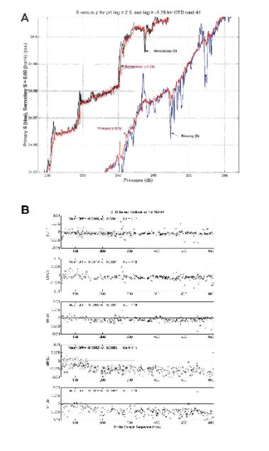 Figure 3. a) Plot of primary (blue) and secondary (black)
salinity with no lags and in red with the lags +2.5 scans and
-1.25 scans that minimize spiking. The secondary salinity
has been offset by 0.02 to facilitate comparison. Data from
CTD cast 41. b) Differences between CTD primary and
secondary and bottle values for CTD casts 8 through 41.
Primary sensor set variables denoted by 0, secondary by 1.
Note apparent shift in C and S near sample 158 (cast 30).
facilitate comparison. Data from CTD cast 41.
Figure 3. a) Plot of primary (blue) and secondary (black)
salinity with no lags and in red with the lags +2.5 scans and
-1.25 scans that minimize spiking. The secondary salinity
has been offset by 0.02 to facilitate comparison. Data from
CTD cast 41. b) Differences between CTD primary and
secondary and bottle values for CTD casts 8 through 41.
Primary sensor set variables denoted by 0, secondary by 1.
Note apparent shift in C and S near sample 158 (cast 30).
facilitate comparison. Data from CTD cast 41.
Table 1. The means and 95% confidence limits of the means of the differences between primary and secondary T and C data and the bottle C and S for the two groups of CTD casts. Note that the shift in both primary and secondary conductivity to lower readings relative to the bottle values between the two groups of casts is significant at the 95% confidence level.
Difference |
Mean (8-28) |
95% CL |
Mean (30-130) |
95% CL |
Difference of Means |
T0-T1 |
-0.0007 |
0.0003 |
-0.0010 |
0.0002 |
0.0003 |
C0-C1 |
-0.0005 |
0.0003 |
-0.0016 |
0.0002 |
0.0011 |
S0-S1 |
+0.0001 |
0.0003 |
-0.0011 |
0.0001 |
0.0012 |
S0-Sb |
-0.0019 |
0.0005 |
-0.0059 |
0.0002 |
0.0040 |
S1-Sb |
-0.0019 |
0.0005 |
-0.0048 |
0.0002 |
0.0029 |
C0-Cb0 |
-0.0014 |
0.0004 |
-0.0044 |
0.0002 |
0.0030 |
C1-Cb1 |
-0.0014 |
0.0003 |
-0.0037 |
0.0002 |
0.0023 |
Based on these CTD/CMiPS and CTD/bottle comparisons, the following steps should be taken in producing the final NBP0204 CTD data set:
1) set conductivity lags for raw 24 Hz CTD data (+2.5 scans for C0, -1.25 scans for C1);
2) for casts 1-28, add +0.0014 to C0 and C1;
3) for casts 30-130, add +0.0044 to C0, and add +0.0037 to C1;
4) compute salinity and other derived variables (i.e., sigma-t) for each scan using Matlab code;
5) lag DO 15 sec with respect to pressure to account for the delay time introduced by the tubing between T/C and DO cells;
6) construct depth-bin averaged data from the 24-Hz data above if desired; and
7) use secondary sensor T1/C1/S1 data for final scientific analysis.
Following these steps should reduce the mean measurement error in the final CTD salinity data to less than +/- 0.001.
On all but the CTD/Rosette casts made in Gerlache Strait, water samples were taken from a minimum of five Niskin bottles to a maximum of all the bottles tripped on a cast for dissolved oxygen determinations. The oxygen samples were always the first taken from the Niskin bottles and were fixed with manganese chloride and sodium iodate/sodium hydroxide reagents immediately after being drawn. The fixed samples were titrated usually within 24 hours of collection, using an automated amperometric oxygen titrator developed at Lamont-Doherty Earth Observatory.
A total of 578 water samples were taken from 56 casts for dissolved oxygen measurements. Of these, all but two stations returned usable data. The samples that provided questionable results were from two stations in Crystal Sound. The problem was determined to be that the manganese chloride dispenser was not delivering the appropriate aliquot of reagent. Changing the dispenser fixed this problem.
Comparison of the dissolved oxygen concentration from the titrated samples with the corresponding values from the oxygen sensor on the CTD showed a tight linear relationship (r2 = 0.9912, see Figure 4a). This relationship was obtained after removing the data from the data points from the Crystal Sound stations that fell well outside of the range of the other data points. The estimated linear relationship between the titrated dissolved oxygen concentration and that obtained from the CTD-mounted sensor is:
O2 = 1.1412 O2(CTD sensor) - 0.174
The estimate for the intercept departed significantly from 0 and the slope of the relationship also departed significantly from the expected value of 1 (Figure 4a), indicating that the titration and/or sensor data are biased.
Examination of the dissolved oxygen concentrations obtained from the CTD sensor and those from the titrations showed that the values measured with the CTD sensor are always lower (Figure 4b). The result is a consistent positive offset between the two dissolved oxygen concentrations (Figures 4a, b). Further comparison with historical data and data from the previous U.S. SO GLOBEC cruises show that the values from the CTD oxygen sensor are low. In particular, the surface dissolved oxygen concentrations are remarkably lower than the historical and previous SO GLOBEC observations. Thus, the conclusion is that the CTD oxygen sensor is measuring lower than the actual dissolved oxygen concentration.
The difference in the titrated and CTD-derived oxygen concentrations plotted as a function of temperature provides an approach for correcting the CTD-derived oxygen values. Temperature provides a proxy for depth, with warmer values representing deep values and coldest values being at the surface. The dissolved oxygen concentration offset at warm temperature (deeper depths) is about 0.2 ml/L to 0.4 ml/L. This offset is relatively constant until temperatures below 0 C are encountered, which occurs at about 130 m to 80 m. At this point, the offset increases to 0.5 ml/L to almost 1.0 ml/L at freezing (-1.84 C). Thus, the offset in dissolved oxygen concentration is clearly nonlinear and is a function of temperature, depth or both. As a result, correction of the CTD-derived dissolved oxygen profiles will require additional effort beyond the standard linear regression. This will be done as part of the post-cruise data quality control and calibration processes.
XBT Probes. Underway observations of the vertical temperature distribution were made with eXpendable Bathythermograph (XBT) probes. The XBT probes were used during the initial crossing of Drake Passage, along a transect through Bransfield Strait and Gerlache Strait, on transits to rendezvous with the L.M. Gould, and on transits to move the L.M. Gould between process sites (Appendix 4).
 Figure 4. a) Comparison of dissolved oxygen concentrations measured by the CTD
oxygen sensor at specific depths versus those measured from titration of discrete
water samples at the same depths (diamonds). The linear fit to these data is shown
as is the regression line equation and correlation coefficient for the relationship.
The squares and corresponding line indicate the one-to-one relationship. b)
Comparison of the dissolved oxygen concentration obtained from titrated samples
(squares) taken from specific depths with that obtained from the CTD oxygen
sensor (diamonds) at the same depth. The difference between the titrated and
CTD-derived oxygen values is also shown (diamonds). The values are plotted as a
function of the temperature at the depth from which the samples were taken.
Figure 4. a) Comparison of dissolved oxygen concentrations measured by the CTD
oxygen sensor at specific depths versus those measured from titration of discrete
water samples at the same depths (diamonds). The linear fit to these data is shown
as is the regression line equation and correlation coefficient for the relationship.
The squares and corresponding line indicate the one-to-one relationship. b)
Comparison of the dissolved oxygen concentration obtained from titrated samples
(squares) taken from specific depths with that obtained from the CTD oxygen
sensor (diamonds) at the same depth. The difference between the titrated and
CTD-derived oxygen values is also shown (diamonds). The values are plotted as a
function of the temperature at the depth from which the samples were taken.
On each of these transects, XBTs were dropped at 10-nm intervals. Two types of XBT probes were used: T-7 probes which go to 760 m, and T-4 probes which go to 460 m. The choice of a particular probe was dictated by the bottom depth.
The majority of the XBTs were launched over the stern of the ship from the main deck using a hand-held launcher. The only exceptions were those dropped in Drake Passage during the initial transit to the study region. The sea state was such as to preclude launching from the main deck; therefore the XBTs were launched from the 01 deck using a hand-held launcher.
A total of 121 XBTs were used during NBP0204. The wire broke on 49 of the drops before the XBT either hit the bottom or exceeded its maximum depth (Appendix 4). In all these cases, the extensive sea ice cover was to blame for the wire breaking. At these locations, the XBT drops were repeated until all or most of the water column was sampled. The temperature measurements from the partial XBT profiles provide useful information on the upper water column structure.
On 12 of the XBT drops, no data or un-usable (e.g., temperatures too warm) data were obtained. For about half of these, the XBT probe failed. A bad connection at the point where the XBT cable goes through the bulkhead to the hand launched was responsible for the remaining un-usable XBT drops. Cleaning the connectors and re-wiring the connection fixed this problem.
XCTD Probes. The use of XCTD-Deep probes on NBP0204 was limited to two locations in Gerlache Strait and to a transect that extended from Boyd Strait northward across Drake Passage to the 200-nautical mile limit that marks the Argentine Exclusive Economic Zone (EEZ) (Appendix 5). On the Drake Passage transect, XCTDs were dropped at 10-nm intervals using a hand-held launcher. It is noteworthy that the XCTDs could be launched over the stern of the N.B. Palmer from the main deck. This is quite unusual for a Drake Passage crossing.
The XCTD-Deep probes have a nominal depth of 1850 m. These probes are designed to be launched at a speed of 3.5 kts. However, the speed of the N.B. Palmer varied between about 3.2 kts and 5.5 kts during a single drop. The deviations from the recommended launch speed altered the final depth reached by the XCTD probe. For most of the XCTDs dropped in Drake Passage the design depth was not reached and most of the drops ended at a shallower depth when all of the wire in the cannister was used.
Few attempts were made to use XCTDs while doing the actual survey grid because of the experiences with using XBTs in the extensive sea ice cover. However, the limited attempts with these probes revealed a problem with the way the cables between the launcher and computer were run through the ship. The XCTD software frequently failed to recognize a probe after is was loaded into the launcher and would abnormally end data acquisition even if the probe was recognized. This resulted in the data from one cast being lost (Appendix 5). A similar problem was encountered on NBP01-03 and was traced to an impedance problem with the cable that runs through the ship. This was supposed to have been fixed by installing a better shielded cable, but was not done. The fix used on this cruise was the same as used on NBP01-03 which was to move the XCTD computer to the wet lab and connect the hand launcher directly to the data acquisition system. After this was done, the XCTDs preformed well and a high-quality data set was collected across Drake Passage.
1.2.3 ADCP Measurements (contributed by Ryan Dorland)
The RDI 153 kHz vessel-mounted Acoustic Doppler Current Profiler (ADCP) on the RVIB N.B. Palmer began recording data at the start of NBP0204 once the Argentine EEZ was passed. Data recording continued throughout the entire survey cruise and ended once the Argentine EEZ was passed on the return transit. The ADCP system records velocity measurements using fifty eight-meter depth bins and five-minute ensemble averages. The current configuration allows for velocity measurements between 31 m and around 400 m, usually less due to rough seas and sea ice conditions.
The ADCP was manually set to bottom track mode whenever water depths were less than 500 m. Bottom tracking was disabled during times when the survey extended beyond the continental shelf edge and into deeper waters for several hours. The RPSC electronics technicians were responsible for switching the ADCP tracking mode.
The ADCP data were processed through CODAS (Common Oceanographic Data Access System) software developed by Eric Firing and Jules Hummon from the University of Hawaii. The N.B Palmer is set up with an automated processing system which includes ship heading corrections from an Ashtech ADU-2 system. Two data sets were produced daily: one with 15-minute averages over the previous 36 hours, and a second with one-hour averages for the entire cruise. These data sets are plotted daily and are available for viewing via the ship's internet system.
Although the ADCP system ran continuously, there were gaps in the data set due to low signal-to-noise ratios produced by interference from the sea ice cover, rough seas, and Ashtech failure. The system was also turned off during a brief stop at Palmer Station. Several spikes appeared in the 1-hour data set, most likely attributable to ship motion not filtered out in preliminary processing. One value determined spurious from the high resolution sets was removed in Crystal Sound for plotting purposes.
The water masses present in the survey grid region are best seen using a potential temperature - salinity (theta - S) diagram constructed from all CTD observations (Figure 5a). Surface waters are at the freezing point, which varies between -1.82 C and -1.84 C, depending salinity. The WW, which is indicated by temperatures colder than -0.5 C and salinity between 34.0 and 34.2 is prominent in the study region. The cold water with salinity between 33.8 and 34.0 was found on the inner shelf and in the polynya along the offshore coast of Adelaide Island.
 Figure 5. a) Potential temperature-salinity diagram constructed
from the CTD collected at the station occupied on the survey grid.
Also shown are the freezing point of seawater as a function of
salinity.(dashed line) and lines of constant potential density
(dotted lines). b) Distribution of the temperature maximum below
200 m constructed from the CTD observations made at the
stations occupied on the survey grid.
Figure 5. a) Potential temperature-salinity diagram constructed
from the CTD collected at the station occupied on the survey grid.
Also shown are the freezing point of seawater as a function of
salinity.(dashed line) and lines of constant potential density
(dotted lines). b) Distribution of the temperature maximum below
200 m constructed from the CTD observations made at the
stations occupied on the survey grid.
Antarctic Surface Water (AASW) was not present at any location. This water mass, which occurs in the upper 80 m is produced by surface heating and mixing process during the austral summer. By the time of NBP0204, this water mass had been eroded, mixed away, and the upper water column cooled to form WW.
Oceanic UCDW appears in the theta-S diagram as a temperature maximum (about 1.5 C to 2.0 C) at a salinity of 34.6. A second temperature maximum of 1.0 C to 1.5 C is found at about the same salinity at stations occupied on the continental shelf. This water is designated Modified CDW and is formed by mixing of the UCDW with the overlying AASW and WW. Offshore of the shelf break at depths of 800 to 1000 m is Lower Circumpolar Deep Water (LCDW) which is distinguished by a salinity maximum of 34.72 at 1.5 C. This water mass was found along the outer shelf and in deep bathymetric features on the shelf. This water mass is the least variable in thermohaline properties of those encountered as evidenced by the tight correlation between temperature and salinity.
The considerable WW layer, surface temperatures at the freezing point, and surface salinities greater than 34.00 are consistent with intense surface cooling and extensive sea ice formation with brine rejection. This is a marked change from the conditions observed during NBP0202 where many sampling sites still had relatively warm water below 30 m and relatively low salinity. Thus, considerable heat was lost from the surface ocean in the six to seven weeks that separated the two cruises.
1.3.2 Water Mass and Circulation Distribution
Temperature Maximum Distribution. The spatial distribution of the the water properties derived from the hydrographic measurements provide an indirect means of determining circulation in the study region. These indirect circulation estimates are augmented by ADCP measurements from the ship.
The distribution of the temperature maximum below 200 m provides a means for tracing the pathways by which oceanic UCDW water moves onto the west Antarctic Peninsula continental shelf. The warm core associated with this water mass retains its identity as the UCDW intrudes onto the shelf below 300 m. The 1.5 C isotherm is used to distinguish the UCDW from shelf water, with temperatures above this indicating oceanic water. The 1.4 C isotherm is associated with west Antarctic Peninsula shelf water. Also, the southern boundary of the ACC is denoted by the 1.8 C isotherm below 200 m.
The distribution of the temperature maximum below 200 m constructed from the NBP0204 observations (Figure 5b) shows an intrusion of UCDW moving onto the shelf north of Alexander Island (between 150 km and 300 km alongshore distance). The 1.5 C isotherm associated with this event extends about 150 km onto the continental shelf. At about 100 km alongshelf distance, a second smaller intrusion is observed at the continental shelf edge.
In the central portion of the survey grid, the 1.4 C isotherm extends almost to the shelf edge. To the north of this, a third intrusion event is occurring in the area overlying Marguerite Trough, which provides a deep connection between the outer shelf and Marguerite Bay. On the shelf side of the 1.5 C isotherm there appears to be an eddy forming at the leading edge of the intrusion as indicated by the pattern of the 1.45 C isotherm.
Another striking feature in the temperature maximum distribution is the presence of the ACC along the edge of the continental shelf. The 1.8 C isotherm is along the shelf edge, except for the southern-most portion of the survey grid. The pattern of the 1.8 C isotherm is suggestive of on- and offshore meanders in the southern boundary of the ACC.
Dynamic Topography Distribution. The dynamic topography, which is the vertical integral of the density anomaly, is a more traditional indicator of circulation which uses the geostrophic balance (horizontal pressure gradients balance the Coriolis acceleration). The vertical density variation in west Antarctic Peninsula continental shelf waters is weak and the shelf is generally less than 500 m deep, which produces a weak dynamic topography. However, a pattern does appear in the dynamic topography calculated at the surface relative to 300 m (Figure 6a).
The dynamic topography shows three regions of closed circulation: at the shelf edge in the southern study region, extending from the shelf edge over the central shelf region, and a large area over the northern part of the survey region. A fourth possible closed region occurs in the inner part of the central study region. The circulation is clockwise around low values of dynamic topography. Thus, each of the regions of closed dynamic topography is characterized by clockwise flow. Flow in the possible fourth region is also clockwise.
An estimate of the speed of this flow is obtained from the horizontal difference of dynamic topography (the units are meters) divided by the horizontal distance and the Coriolis parameter (about 0.0001 s-1). These calculations give flows associated with the clockwise gyres of 5 cm/sec to 10 cm/sec.
ADCP Current Vectors. The ADCP-derived current distribution between 31 m and 50 m (Figure 6b) and between 175 m and 225 m (Figure 7) confirm the flow pattern suggested by the temperature maximum and dynamic topography distributions, although these current vectors show considerable spatial and temporal variability. There is the suggestion of clockwise flow in the outer parts of the southern and central portions of the study region. There is also evidence of a clockwise eddy feature on the northwestern edge of Marguerite Trough in the outer part of the northern study region. The ADCP velocity distributions also show south-southwest flow around the northern tip of Adelaide Island. This flow may be associated with the coastal current that is known to exist in this area. This feature does not appear in the dynamic topography field because the number of hydrographic measurements made in the inner shelf region were insufficient to resolve this feature.
 Figure 6. a) Distribution of the dynamic topography
at the surface relative to 300 m
constructed from the CTD observations made at the stations occupied on the survey grid.
b) One-hour averaged ADCP-derived current vectors for the 31 m to 50 m strata.
Current vectors are computed from data collected at individual station locations. The
extensive sea ice made ADCP data collection problematic during times that the ship was
moving. Figure provided by Ryan Dorland.
Figure 6. a) Distribution of the dynamic topography
at the surface relative to 300 m
constructed from the CTD observations made at the stations occupied on the survey grid.
b) One-hour averaged ADCP-derived current vectors for the 31 m to 50 m strata.
Current vectors are computed from data collected at individual station locations. The
extensive sea ice made ADCP data collection problematic during times that the ship was
moving. Figure provided by Ryan Dorland.
 Figure 7. One-hour averaged ADCP-derived current vectors for the 175 m to 225 m strata.
Current vectors are computed from data collected at individual station locations. The extensive
sea ice made ADCP data collection problematic during times that the ship was moving. Figure
provided by Ryan Dorland.
Figure 7. One-hour averaged ADCP-derived current vectors for the 175 m to 225 m strata.
Current vectors are computed from data collected at individual station locations. The extensive
sea ice made ADCP data collection problematic during times that the ship was moving. Figure
provided by Ryan Dorland.
In general the ADCP-derived currents were weak and variable in the survey area averaging less than 10 cm/s. The exception to this is along the outer shelf edge where the southern boundary of the ACC is present. Current velocities at this location reached 50 cm/s to the northeast.
1.4 Hydrography/Circulation Highlights from all SO GLOBEC Cruises
This is the report of the fourth and final U.S. SO GLOBEC survey cruise and as such it is appropriate to include a short summary of the new things that have been learned about the circulation and hydrography of the west Antarctic Peninsula continental shelf. Some highlights are:
1) Identification of a coastal current that flows to the south-southwest along the offshore side of Adelaide Island;
2) Recognition of the importance of Marguerite Trough as a conduit for bringing oceanic CDW into the inner portion of Marguerite Bay;
3) Recognition of the large-scale influence of the oceanic water masses UCDW and LCDW on the water mass structure on the west Antarctic Peninsula continental shelf;
4) Recognition of the large-scale influence of the oceanic water masses UCDW and LCDW on sea ice formation and extent on the west Antarctic Peninsula continental shelf;
5) Recognition of the importance of the Antarctic Circumpolar Current in determining the water mass structure on the west Antarctic Peninsula continental shelf;
6) Identification of a closed gyre in the northern portion of the region surveyed during the U.S. SO GLOBEC cruises; and
7) Recognition that other regions of closed circulation may occur at other locations on the continental shelf covered during the survey cruises.
Much credit for the high quality hydrographic observations collected during NBP0204 goes to the RPSC marine technicians Nancy Ford, Jamee Johnson and Stian Alesandrini, and the electronic technicians, Fred Stuart and Todd Johnson. Their willing and cheerful response to all requests made collection of these data a pleasure. We also appreciate the efforts of the winch operators Sam Villanueva, Bienvenido (Ben) Aaron, Lauro Garde, and Enrique (Ricky) Alveco, who endured cold tedium in the Baltic Room to obtain these data. Their cheerful attitudes made the long hours in the Baltic Room pass more quickly. We also thank Captain Joe Brokowski, the bridge officers, Mike Watson, Paul Jarkiewicz, Rachelle Pagtalunan, and the ice pilot, Vladimir Repin for skillful ship handling, which got us to our stations and made it possible to safely deploy and retrieve instruments. To all of these individuals, we extend our deepest thanks.
2.0 Microstructure Measurements with CMiPS
(Bob Beardsley and Chris MacKay)
One of the original objectives of the U.S. Southern Ocean GLOBEC physical oceanographic program was to investigate the flow of relatively warm, saline Upper Circumpolar Deep Water (UCDW) onto the shelf and determine how it mixes with the overlying surface waters that are generally cooler and fresher. The CTD stations made during the NBP0204 broad-scale survey document the water properties over the mid- and outer shelf in the study area and show the primary pathways of UCDW onto the shelf in winter when much of the shelf is covered with ice. The CTD stations made close to Adelaide Island document the water properties in this partially open area.
The Palmer’s CTD was equipped with a precision pressure sensor and two independent temperature/conductivity sensor sets which were sampled and recorded at 24 Hz. Two CTD cast profiles were generally used: a) for some casts when the FRRF instrument was mounted on the CTD, the lowering speed was 10 m/min to 50 m, 20 m/min to 100 m, then 40 m/min to the bottom; and b) for all other casts, the lowering speed was 20 m/min to 20 m, then 40 m/min to the chosen depth or bottom. At a lowering speed of 40 m/min, the CTD recorded data every 2.8 cm. While the 24 Hz temperature (T) and conductivity (C) data capture much of the fine-scale variability, the time lags inherent in the ducted flow-through design of the TC sensor set tend to smooth the raw data, so that features with vertical scales less than roughly 30 cm are not well resolved.
To investigate mixing processes, temperature and conductivity must be measured on a much finer vertical scale. To do this, a new self-contained instrument called CMiPS (CTD-mountable Microstructure Profiling System) was attached to the CTD rosette and used to collect high-resolution T, C, and pressure profile data. With a sample rate of 512 Hz and a lowering speed of 40 m/min, CMiPS records data every 0.1 cm in the vertical. Analysis of the fluctuations of temperature and conductivity on these short scales (called 'microstructure') will provide evidence if turbulent mixing is occurring somewhere in the water column and how homogeneous are different layers.
CMiPS was used for the first time on NBP0202 and some of its early ‘teething’ problems were identified and fixed during that cruise. However, most of NBP0202 was conducted in open water, so that the CMiPS (and CTD) data include the wave-induced ship’s motion, which was large enough on many stations to cause the instrument to stop and reverse direction (rise) frequently on the down cast. Both CTD and CMiPS are designed to see clear flow during the down cast without any turbulence created when the instrument is stopped and raised up through its own wake, even if only for a few seconds. The presence of these self-wake effects in the CMiPS data makes the interpretation of the NBP0202 microstructure data difficult.
This cruise (NBP0204) was conducted almost entirely in ice or small leads surrounded by ice.
As a result, there was very little ship motion for most of the cruise and the CTD and CMiPS were lowered with no vertical reversals at all stations, even when using the 10 m/min lowering speed near the surface. These were thus ideal conditions for using CMiPS to measure microstructure.
Indeed, an initial look at the CMiPS data shows many small (< 1m) steps in the main thermocline and deeper, suggesting that significant mixing could be occurring throughout the water column.
The CMiPS group on this cruise consisted of Chris MacKay and Bob Beardsley aboard the Palmer and Laurie Padman and Rolf Lueck ashore who advised on data processing and interpretation and instrument issues. All played critical roles in getting a marvelous microstructure data set from CMiPS during NBP0204. Other supporting members include: Eileen Hofmann, Baris Salihoglu, Sue Beardsley, Francisco Viddi, Gustavo Thompson, Jamee Johnson, Nancy Ford, Stian Alesandrini, Fred Stuart, Todd Johnson, Sam Villanueva, Bienvenido (Ben) Aaron, Lauro Garde, and Enrique (Ricky) Alveco.
2.2 Instrumentation and Data Collection
CMiPS is a self-contained instrument that samples two fast-response thermistors, a SeaBird SBE 7 micro-conductivity sensor, and a high-resolution pressure sensor at 512 Hz and stores the data on a solid-state disk inside the instrument. The sensors are mounted on the tip of a cone that attaches to one end of the cylindrical electronics pressure case (Figure 8a). Power is provided by a separate cylindrical battery case, which has an off/on switch that is used to turn on CMiPS as the CTD is being launched and turn it off when the CTD is back on deck. On this cruise, CMiPS was mounted vertically on the rosette frame with its sensors oriented facing down and located near the bottom of the frame so that the flow to the CMiPS sensors was as uninterrupted as possible (Figure 8b). This placed the CMiPS sensors on the opposite side of rosette from the CTD sensors (Figure 8c). The battery cast was mounted on the other side of the rosette to provide flow and weight symmetry.
A total of 130 CTD casts were made on NBP0204. CMiPS was used on most of these casts, with a few exceptions when the instrument was removed from the rosette for repair or the water depth was greater than the 2000 m limit for CMiPS (Table 2). The typical protocol at each station was: a) soak the CTD/CMiPS at 10 m for 3-6 minutes to cool off the sensors; b) make a CMiPS cast from the surface to a depth of 300-400 m at 40 m/min below 20 m, followed by a quick return at 50 m/min to the surface; c) make a second cast with CMiPS to the bottom, collecting water samples on the up cast back to the surface; and d) download the CMiPS data onto a laptop and place the raw data on the ship’s science disk. If the bottom depth was less than 500 m, the FRRF instrument was mounted on the CTD rosette and the slower lowering rate was used (10 m/min to 50 m, 20 m/min to 100 m, then 40 m/min to the bottom). At 8 stations, additional CTD/CMiPS casts were made to look at the temporal and spatial variability between the repeat casts. These multiple-cast stations are called here ‘anchor stations’, although the ship was usually parked in ice next to a lead or a small hole the Palmer had made on her starboard side to get the CTD into the water. The locations of CMiPS casts are shown in Figure 8d.
CMiPS records raw data in blocks from the time it is turned on (just before launching) to the time it is turned off (when the instrument is recovered and back on deck). The first block starts when the instrument is turned on, but subsequent blocks all start on the hour, with a header indicating the start time of each block. CMiPS has a storage capacity of roughly 4 hrs, so for the longer stations (either deep or repeated casts), several blocks were usually recorded (Table 2).
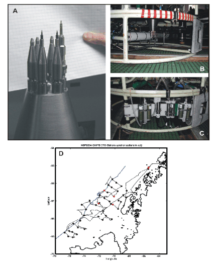 Figure 8. a) CMiPS sensors mounted on the bottom of cone. The two
thermistors and the micro-conductivity probe are spaced 60 degrees
apart on the circle with 0.81 inches radius. The tip of the micro-conductivity probe leads the plane of the thermistors by about 1 cm.
The other sensor mounts hold dummy heads. b) CMiPS mounted to
rosette with sensors about 17 cm above the bottom of the rosette. A
piece of duct tape was attached to the CTD frame to minimize vortex
shedding and flow distortion that could introduce flow noise in the
CMiPS data. c) The CTD primary (left) and secondary (right) T/C
sensor sets. A SBE dissolved oxygen sensor was mounted inline
between the primary sensor set and its pump. These CTD sensors
were located opposite the CMiPS sensors. d) Map showing locations
of CTD/CMiPS casts. The anchor stations are shown in red.
Additional casts and two anchor stations were made in Gerlache Strait,
located off this map. The heavy blue curve is the 1000–m isobath.
Figure 8. a) CMiPS sensors mounted on the bottom of cone. The two
thermistors and the micro-conductivity probe are spaced 60 degrees
apart on the circle with 0.81 inches radius. The tip of the micro-conductivity probe leads the plane of the thermistors by about 1 cm.
The other sensor mounts hold dummy heads. b) CMiPS mounted to
rosette with sensors about 17 cm above the bottom of the rosette. A
piece of duct tape was attached to the CTD frame to minimize vortex
shedding and flow distortion that could introduce flow noise in the
CMiPS data. c) The CTD primary (left) and secondary (right) T/C
sensor sets. A SBE dissolved oxygen sensor was mounted inline
between the primary sensor set and its pump. These CTD sensors
were located opposite the CMiPS sensors. d) Map showing locations
of CTD/CMiPS casts. The anchor stations are shown in red.
Additional casts and two anchor stations were made in Gerlache Strait,
located off this map. The heavy blue curve is the 1000–m isobath.
Table 2. Table listing CTD/CMiPS cast number, station number or name, the time in decimal yearday at the bottom of the cast, the water depth, and the maximum depth of the cast. The 12 casts where the CMiPS and CTD were not processed and merged during the cruise are denoted by the NaN for cast depth.
CTD Cast Number |
Station Number |
YDay (GMT) |
Longitude (DD) |
Latitude (DD) |
Water Depth (m) |
Cast Depth (db) |
9 |
Transit 1 |
221.6389 |
-70.5498 |
-67.1877 |
505 |
205 |
10 |
Transit1 |
221.6576 |
-70.5515 |
-67.1886 |
1610 |
NaN |
11 |
75 |
223.884 |
-76.1688 |
-68.6713 |
2133 |
NaN |
12 |
76 |
224.3562 |
-75.6975 |
-68.7486 |
468 |
202 |
13 |
76 |
224.3743 |
-75.6945 |
-68.7487 |
467 |
454 |
14 |
77 |
224.8681 |
-75.1206 |
-68.8777 |
514 |
205 |
15 |
77 |
224.891 |
-75.1186 |
-68.8739 |
501 |
477 |
16 |
to 81 |
225.5028 |
-75.6338 |
-69.0528 |
370 |
294 |
17 |
to 81 |
225.5194 |
-75.6309 |
-69.0518 |
365 |
347 |
18 |
81 |
225.8576 |
-76.3166 |
-69.0041 |
420 |
204 |
19 |
81 |
225.8736 |
-76.3113 |
-69.0029 |
410 |
396 |
22 |
74 |
227.0146 |
-75.6445 |
-68.2748 |
1710 |
102 |
24 |
73 |
227.3875 |
-75.0172 |
-68.4657 |
429 |
NaN |
25 |
73 |
227.4042 |
-75.0151 |
-68.4642 |
431 |
NaN |
26 |
72 |
227.8187 |
-74.0702 |
-68.5881 |
683 |
NaN |
27 |
72 |
227.8299 |
-74.0705 |
-68.5877 |
681 |
NaN |
28 |
72 |
227.8562 |
-74.0712 |
-68.5873 |
682 |
NaN |
29 |
65 |
229.625 |
-74.7061 |
-68.0857 |
410 |
NaN |
30 |
65 |
229.6431 |
-74.7007 |
-68.0852 |
404 |
NaN |
32 |
43 |
232.6354 |
-72.4704 |
-67.2211 |
413 |
252 |
33 |
43 |
232.6549 |
-72.4686 |
-67.218 |
413 |
392 |
34 |
44 |
233.4875 |
-73.4 |
-66.9917 |
3410 |
1994 |
35 |
45 |
234.0715 |
-74.4879 |
-67.209 |
2971 |
2002 |
36 |
46 |
234.866 |
-73.8001 |
-67.4582 |
438 |
NaN |
37 |
46 |
234.8854 |
-73.8004 |
-67.4562 |
444 |
425 |
41 |
62 |
236.6708 |
-74.1782 |
-67.8172 |
1091 |
1085 |
42 |
48 |
237.3736 |
-72.2429 |
-67.8967 |
303 |
199 |
43 |
48 |
237.391 |
-72.238 |
-67.8947 |
303 |
291 |
44 |
49 |
237.7604 |
-71.6021 |
-68.076 |
463 |
202 |
45 |
49 |
237.7826 |
-71.597 |
-68.0734 |
431 |
429 |
46 |
40 |
238.575 |
-70.396 |
-68.0334 |
863 |
200 |
47 |
40 |
238.5979 |
-70.396 |
-68.0334 |
863 |
830 |
48 |
41 |
240.4271 |
-71.241 |
-67.833 |
375 |
350 |
49 |
41 |
240.4465 |
-71.2396 |
-67.8308 |
380 |
361 |
50 |
26 |
241.4694 |
-72.0043 |
-67.1236 |
424 |
397 |
51 |
26 |
241.4903 |
-72.0037 |
-67.1252 |
425 |
406 |
52 |
26 |
241.7722 |
-72.1394 |
-67.1222 |
426 |
302 |
53 |
26 |
241.7847 |
-72.1425 |
-67.1248 |
426 |
304 |
54 |
26 |
241.7979 |
-72.1457 |
-67.1276 |
426 |
304 |
55 |
26 |
241.8104 |
-72.1492 |
-67.1304 |
429 |
305 |
56 |
4 |
244.4035 |
-69.101 |
-66.1583 |
344 |
300 |
57 |
4 |
244.4215 |
-69.1041 |
-66.1572 |
347 |
327 |
58 |
3 |
244.7965 |
-69.8171 |
-65.9555 |
345 |
204 |
59 |
3 |
244.8132 |
-69.8186 |
-65.9517 |
345 |
339 |
60 |
2 |
245.1111 |
-70.2918 |
-65.783 |
748 |
814 |
64 |
12 |
246.5417 |
-70.8689 |
-66.091 |
899 |
895 |
65 |
11 |
246.8861 |
-70.3944 |
-66.2271 |
467 |
206 |
66 |
11 |
246.9028 |
-70.3956 |
-66.2267 |
467 |
446 |
67 |
10 |
247.4299 |
-69.6239 |
-66.4551 |
503 |
350 |
68 |
10 |
247.4521 |
-69.6216 |
-66.4538 |
503 |
484 |
69 |
16 |
247.7917 |
-70.1675 |
-66.7506 |
519 |
332 |
70 |
16 |
247.8035 |
-70.1683 |
-66.7496 |
517 |
351 |
71 |
16 |
247.8181 |
-70.1692 |
-66.7488 |
516 |
358 |
72 |
16 |
247.8313 |
-70.1699 |
-66.748 |
515 |
365 |
73 |
16 |
247.8458 |
-70.1709 |
-66.7472 |
516 |
358 |
74 |
15 |
247.866 |
-70.1714 |
-66.7465 |
519 |
497 |
75 |
15 |
248.4694 |
-70.9625 |
-66.5146 |
543 |
356 |
76 |
14 |
248.4882 |
-70.9593 |
-66.514 |
543 |
523 |
77 |
14 |
248.716 |
-71.367 |
-66.4018 |
791 |
371 |
78 |
14 |
248.7306 |
-71.3654 |
-66.3991 |
814 |
378 |
79 |
14 |
248.7451 |
-71.3636 |
-66.397 |
835 |
377 |
80 |
14 |
248.7597 |
-71.3607 |
-66.3952 |
847 |
378 |
81 |
23 |
248.8132 |
-71.3555 |
-66.3913 |
871 |
866 |
82 |
23 |
249.3125 |
-71.9969 |
-66.6859 |
1688 |
350 |
83 |
22 |
249.3542 |
-71.9908 |
-66.6823 |
1767 |
1756 |
84 |
22 |
249.6847 |
-71.4295 |
-66.8222 |
478 |
366 |
85 |
21 |
249.7035 |
-71.4282 |
-66.8205 |
478 |
460 |
86 |
21 |
250.2778 |
-70.7032 |
-67.0401 |
501 |
353 |
87 |
20a |
250.2986 |
-70.7014 |
-67.039 |
504 |
484 |
88 |
20a |
250.6056 |
-70.282 |
-67.206 |
662 |
350 |
89 |
20a |
250.6215 |
-70.2794 |
-67.2065 |
663 |
351 |
90 |
20a |
250.6306 |
-70.2769 |
-67.2067 |
664 |
153 |
91 |
19 |
250.6486 |
-70.2744 |
-67.2068 |
663 |
641 |
92 |
19 |
250.9389 |
-69.5162 |
-67.4732 |
383 |
NaN |
93 |
18 |
250.9542 |
-69.5149 |
-67.473 |
390 |
NaN |
94 |
18 |
251.6243 |
-69.1438 |
-67.0468 |
391 |
351 |
95 |
17 |
251.6431 |
-69.1437 |
-67.0479 |
427 |
419 |
96 |
17 |
252.1486 |
-69.5015 |
-66.9962 |
526 |
352 |
97 |
9 |
252.1701 |
-69.5046 |
-67.0017 |
512 |
495 |
98 |
9 |
252.5396 |
-68.9018 |
-66.6783 |
332 |
300 |
99 |
8 |
252.5556 |
-68.9067 |
-66.6802 |
328 |
311 |
100 |
8 |
252.7722 |
-68.4363 |
-66.8124 |
70 |
67 |
101 |
5 |
252.7806 |
-68.4373 |
-66.8126 |
73 |
66 |
102 |
5 |
253.2639 |
-68.4083 |
-66.4239 |
693 |
350 |
103 |
RI1 |
253.2833 |
-68.4105 |
-66.4276 |
675 |
650 |
104 |
RI1 |
254.4056 |
-65.5751 |
-65.1841 |
622 |
400 |
105 |
RI2 |
254.4215 |
-65.5711 |
-65.1839 |
558 |
401 |
106 |
RI2 |
254.6653 |
-65.5921 |
-65.1656 |
714 |
400 |
107 |
RI3 |
254.6868 |
-65.589 |
-65.1639 |
723 |
730 |
108 |
RI3 |
254.8924 |
-65.5464 |
-65.1512 |
595 |
351 |
109 |
RI3 |
254.9056 |
-65.5422 |
-65.1497 |
557 |
352 |
110 |
RI3 |
254.9187 |
-65.539 |
-65.1487 |
549 |
350 |
111 |
RI4 |
254.9375 |
-65.5352 |
-65.1473 |
536 |
532 |
112 |
RI4 |
255.1208 |
-65.5098 |
-65.1317 |
533 |
354 |
113 |
RI4 |
255.1347 |
-65.5091 |
-65.1302 |
546 |
355 |
114 |
RI5 |
255.1542 |
-65.5092 |
-65.1289 |
553 |
500 |
115 |
RI5 |
255.2882 |
-65.5023 |
-65.1234 |
537 |
353 |
116 |
GS1 |
255.3076 |
-65.5016 |
-65.1235 |
536 |
501 |
117 |
GS1 |
256.8396 |
-63.0305 |
-64.7169 |
369 |
352 |
118 |
GS1 |
256.8528 |
-63.0283 |
-64.7166 |
372 |
352 |
119 |
GS2 |
256.9326 |
-62.6609 |
-64.5782 |
757 |
350 |
120 |
GS2 |
256.9542 |
-62.6598 |
-64.5782 |
759 |
738 |
121 |
GS3 |
257.0389 |
-62.2346 |
-64.4683 |
656 |
350 |
122 |
GS3 |
257.0528 |
-62.2352 |
-64.4682 |
656 |
351 |
123 |
GS3 |
257.0715 |
-62.2341 |
-64.4682 |
662 |
642 |
124 |
GS4 |
257.1576 |
-61.9416 |
-64.3103 |
1035 |
350 |
125 |
GS4 |
257.1799 |
-61.9419 |
-64.31 |
1042 |
899 |
126 |
GS4 |
257.1938 |
-61.9431 |
-64.3102 |
1060 |
434 |
127 |
GS4 |
257.2174 |
-61.9432 |
-64.3103 |
1055 |
1049 |
128 |
GS5 |
257.3264 |
-61.8673 |
-64.1669 |
718 |
500 |
129 |
GS5 |
257.3493 |
-61.8672 |
-64.1668 |
718 |
695 |
130 |
GS6 |
257.4681 |
-61.7538 |
-64.0066 |
1204 |
1178 |
Following each series of casts at a station, the CMiPS raw data files were transferred to a laptop and a series of Matlab programs run to a) convert the CMiPS raw binary data files into mat-files, b) merge the files which cover the set of casts just made, c) convert the CMiPS data into scientific units, and d) merge the CMiPS processed and 24 Hz CTD data for each cast into its own single mat-file called CMiPSctdxxx, where xxx indicates the cast number. This approach was taken to facilitate analysis during the cruise and provide others with all the important data for a single CTD/CMiPS cast together. Of the 113 CTD/CMiPS casts made during the cruise, data from all but 12 casts were processed in this way. The unprocessed casts are denoted by the NaN in the right hand column in Table 2.
The CMiPS raw data include pressure (P), pre-emphasized pressure (Ph), temperature (T), thermistor 1 pre-emphasized temperature (T1h), thermistor 2 pre-emphasized temperature (T2h), and pre-emphasized conductivity (Ch). The converted CMiPS data includes time (t) from start of the station, thermistor 1 and 2 high-resolution temperatures (T1_hr, T2_hr), high-resolution conductivity (C_hr), and high-resolution pressure (P_hr). The conversion from raw counts to scientific units requires comparing the CMiPS data with CTD data to determine scaling factors for the high-resolution pressure, temperatures and conductivity. An interactive Matlab program was used to compare the two data sets from a cast and pick appropriate scaling factors, which were then put back into the conversion programs, so subsequent CMiPS data would be correctly scaled. New temperature and conductivity scaling factors were determined after a new thermistor or conductivity probe were mounted on CMiPS. Most of the CMiPSctdxxx files include both the raw and the converted and scaled CMiPS data. This approach of placing the raw and converted CMiPS and raw CTD data for each cast in a single file was taken to facilitate analysis both during the cruise and post-cruise.
After the last CTD/CMiPS cast was made, the raw and processed CMiPS data, the 24 Hz CTD data, and the merged CMiPSctdxxx files were put in directories on one of the ship’s UNIX machines and DAT tapes were made of the zipped files. In addition, the raw unzipped CMiPS data were put onto 3 CD-R disks. Copies of the raw and processed CMiPS data, the 24-Hz CTD data, and the CMiPSctdxxx files were stored on a removable hard disk for additional backup.
Following each set of casts, plots of the raw and scaled CMiPS data were made and compared with the 24 Hz CTD data to help monitor CMiPS performance as well as for later scientific analysis. Problems with the CMiPS temperature and conductivity sensors and/or supporting electronics were easily seen in both sets of plots. This rapid analysis allowed decisions about repair work to be done efficiently with a minimum of instrument down time and missed stations. Sections (150 sec) of raw CMiPS and CTD data were sent by email to Laurie Padman and Rolf Lueck for their inspection and analysis and help in diagnosing instrument problems.
None of the problems were major and they were focused on three areas of the instrument. The first was a software problem related to increasing the gain in the instrument by a factor of four since the earlier NBP0202 cruise. This caused random creation of new data files, often without any loss of continuous data. This problem only occurred when one or more sensors produced signals outside of the input range of the A/D converter. There were also problems with several connectors making reliable connections in the oil-filled nose. These components were replaced with a different type of connector and a cleaning step was added during probe installation. The final difficulty with the instrument has been a problem with pressure- and temperature-related expansion and contraction of the oil in the nose, over-stressing a rubber diaphragm that separates the oil from the outside sea water. This diaphragm is designed to expand within the cone as the instrument is lowered, thus equalizing the pressure in the oil with that outside the cone. This has at various times allowed small amounts of water into the nose cavity which has cause noise on some of the sensors and a small seepage of oil out of the nose cavity, which contaminates the micro-conductivity sensor, causing a loss in sensitivity. This was controlled during the cruise by servicing the nose when required and regular cleaning of the conductivity sensor in Triton solution between casts. This problem will be solved by further investigation of the properties of selected oils and diaphragms.
The initial objectives of NBP0204 were to help position the Gould for her ice-drift stations and make measurements along the large-scale survey grid established in past SO GLOBEC survey cruises. Due to the heavy ice cover over the mid-shelf, the Palmer focused her survey work on the stations located along the outer shelf. At most of these stations, a pair of CTD/CMiPS casts was made (Figure 8b). At four “anchor stations” in the grid, additional casts were made to investigate water column variability and microstructure in more detail. Descriptions of the anchor station sampling follow.
2.5.1 Anchor Station 1: Repeat CTD/CMiPS casts were made on August 29 with the Palmer parked against the ice along a long but narrow lead near the mid-shelf. Casts 52, 53, 54, and 55 were made at approximately 20 min spacing to a depth of 300 m. Both CTD and CMiPS returned good data.
The CTD t2 (T), s2 (S), and sigma-t2 (D) profiles show significant variability between casts. The surface mixed layer became more uniform with depth after 52, with the base at T = -1.828 +/- 0.002 deepening from 58 m (53) to 70 m (54-55). T increased only slightly +0.02 down to 85 m on all casts, where the main thermocline started. S and D have the same structure.
The main thermo-, halo-, and pycno-clines started at the base of the SML, were strongest above 150 m, and decreased in slope down to 300m. The clines were displaced vertically by roughly +6 m (52-53), + 2 m (53-54), and -5 m (54-55), corresponding to vertical velocities w of order 0.5 cm/s. The variation between 54-55 suggests that the vertical displacement was due to a second-mode internal wave, with w = 0 about 140 m. The N2 profile at 55 increased from 0 starting at 75 m to a maximum of about 0.011 s-1 (10 min period) near 110 m, then decreased smoothly to about 0.002 s-1 at 250 m.
A few features can be traced from one cast to another. Examples include: a) a 3-m thick mixed layer centered around 177 m seen in 52 is seen in 53; b) a 0.02 sigma-t step at 95 m in 52 remains distinct to 54; a 3-m thick layer at 95 m in 53 is partially smeared in 54. However, many small scale features seen on one cast do not appear in the other casts. Assuming a 20 cm/s ship/ice drift relative to the deeper flow, the horizontal distance between casts is roughly 20 minutes x 20 cm/s = 240 m; most features have shorter horizontal extent.
One striking feature is the change in sigma-t on a pressure surface between 54 and 55. While the change in profile could be explained by a mode-2 internal wave, beneath 160 m there is a 0.01 difference, which would mean a 6 cm/s current change over a 20-m depth change (assuming a horizontal distance of 240 m between casts and a thermal-wind balance). It is unlikely the currents are in geostrophic balance over this scale, so it is more likely due to internal wave motions and spatial variability.
2.5.2 Anchor Station 2: Repeat CTD/CMiPS casts were made on September 4 with the Palmer parked against the ice along a twisting lead at about -66 45' S, -70 10' W. Six repeat casts were made, starting with 69 at 1843 GMT and ending with 74 starting down at 2027 GMT, with an average spacing of 20.2 min. During this period, the ship drifted about 517 m SW, an average speed of 8.5 cm/s. The water motion relative to the ship was measured with the ADCP so as to provide a length scale between successive casts. With clear and sunny skies, winds were weak and towards the SW during this period. The first five casts were made to an average depth of 350 m, while the last cast was a full-depth cast to 498 m and collected water samples on the up-cast. The CTD and CMiPS returned good data for all casts.
As was found at Anchor Station 1, the CTD t2(T), s2(S), and sigma-t2(D) profiles at Anchor Station 2 exhibit clear differences in vertical structure from cast to cast (Figures 9a, b, c). The surface mixed layer (SML) depth varied from 62 to 75 m, with large variations in the T and S in the ~10 m transition layer between the bottom of the SML and the top of the main thermo- and haloclines. Figures 10a, b show CMiPS high-resolution temperature T2_hr and conductivity profiles for the depth range 68-77 m. Note the large differences in structure between casts. The CMiPS temperature profile for cast 70 shows two nearly isothermal layers separated by a sharp jump in temperature at 72.8 m. The temperature increased by 0.1 C over 10 cm, giving a gradient of 1 C/m. A similar sharp jump in conductivity occurred at this interface. Sharper gradients can be found on even smaller scales.
The main thermo-, halo-, and pycno-clines extended down to about 250 m, with the maximum gradients in the 90-110 m range. T and S are mostly monotonic with depth, with layers of nearly constant T and S varying from < 1 m to a few m thick occurring at different depths during the cast. Some of these features can be traced from cast to cast, but not easily nor without change.
It appears that no simple vertical shifting of T and S as by a mode-1 internal wave explains the observed cast-to-cast variability.
2.5.3 Anchor Station 3: Anchor Station 3 was made on September 5 at Station 14 under ideal weather conditions; there was excellent visibility with a high cloud bank so that we could see the sun on Adelaide Island and -10 to -5 C air temperatures with very weak winds. The Palmer was parked in a small lead, surrounded by icebergs. On the transit to this station, we noticed that sea smoke was rising in the open area around many icebergs, suggesting that these regions, although perhaps small in area, could be contributing significantly to the local heat flux, cooling the surface waters. Due to the 2-m swell from offshore, many of the icebergs appeared to be bobbing, which would also enhance melting and mixing around the iceberg. The spatial density of icebergs has increased during the last cross-shelf transect and to this station. Using the Main 1 and Port radars, we measured the distance and size of the large iceberg nearest the ship at the time of the third CTD downcast; the berg was 1.3 nm from the ship, and roughly 240-280 m in diameter. It appeared to have an aspect ratio of 1/5, so the height above water would be roughly 50 m, so it could extend as deep as 50*9 = 450 m. We then counted the number of icebergs clearly shown on the radar image within the 3-nm radius. The total was 1 within 1.3 nm, and 49 within 3 nm. This gives a concentration of crudely 1 iceberg/2 km2. It is unclear what influence being this close to a relatively large iceberg and in a region of icebergs has on the water structure measured at this anchor station.
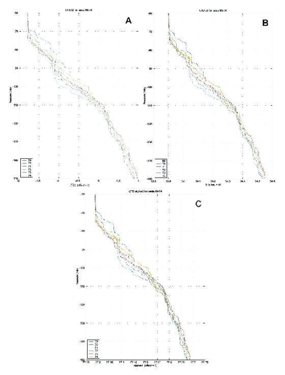 Figure 9. a) CTD secondary temperature (t2) profiles at Anchor Station 2. b) CTD
secondary salinity (s2) profiles at Anchor Station 2. c) CTD secondary sigma-t (sig2)
profiles at Anchor Station 2.
Figure 9. a) CTD secondary temperature (t2) profiles at Anchor Station 2. b) CTD
secondary salinity (s2) profiles at Anchor Station 2. c) CTD secondary sigma-t (sig2)
profiles at Anchor Station 2.
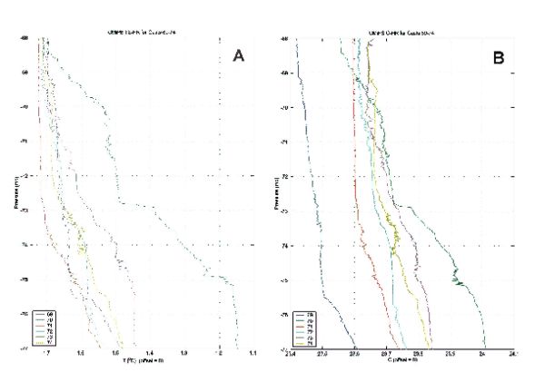 Figure 10. a) CMiPS high-resolution temperature (T2_hr) profiles at Anchor Station 2. b)
CMiPS high-resolution conductivity (C_hr) profiles at Anchor Station 2.
Figure 10. a) CMiPS high-resolution temperature (T2_hr) profiles at Anchor Station 2. b)
CMiPS high-resolution conductivity (C_hr) profiles at Anchor Station 2.
2.5.4 Anchor Station 4: Anchor Station 4 was made at Station 20A in a large lead in dense fog in the center of Marguerite Trough on September 7. The Palmer had been following leads towards Station 20 from 21 over the outer shelf, and the location of 20 was moved to 20A to stay within the lead and over the deepest part of the trough. The Palmer parked at the side of the lead, which was covered by nilas ice with ice flowers in some regions and some open water. The lead was roughly 2.5 nm long and 0.3 nm wide, with the ship located in the center lengthwise. When doing the first CMiPS cast to 350 m, we noticed that the base of the surface layer was very sharp, so we did a second CMiPS cast to 350 m. While doing this, Peter Wiebe reported that BIOMAPER-II was showing a very strong scattering layer at about the base of the surface layer than appeared to have physical and not biological origins, perhaps due to concentrated sound speed gradients. We made a third CMiPS cast between 50 and 150 m, then made the last CTD cast using the FRRF lowering speed protocol to the bottom. The CTD and CMiPS data look excellent.
2.5.5 Anchor Stations 5 and 6: After the Palmer had completed the northern grid in the SO GLOBEC survey area, the decision was made for the Palmer to spend one day sampling around an iceberg before steaming to Palmer Station. In particular, we hoped to do CTD/CMiPS casts close to an iceberg to investigate if the iceberg was influencing the local water around it while the other groups hoped to characterize the biological distributions of target organisms in the vicinity of the iceberg.
The first pair of CTD/CMiPS casts (104-105) were made roughly 1 nm from an iceberg at about 10 GMT on September 11, with the ship at -65 11.04 S, -65 33.86 W at 1043 GMT. Two other icebergs were within 1.5 nm and a total of 11 within 2.5 nm. To keep on the science plan schedule, just two casts were made to 400 m and no water samples were collected. These casts showed considerable structure in the upper 200 m. The ice conditions there were not good for ROV and ice sampling, the next two sets of measurements to be made, so the decision was made to make a MOC1 tow back along the ship's course towards the SW where thicker ice had been observed. Near the end of this tow, the ship passed a small iceberg. When the tow was completed, the ship steamed back to this iceberg and set up for the ROV and ice sampling. The Gould was just completing ice sampling at a site near this iceberg, and reported that the conditions were good for ice that operation. They also suggested that this was an important place for data collection, since the ice had some flooding with interesting biology.
After the Palmer finished its morning ROV and ice sampling, the ship moved closer to this iceberg to make the second pair of CTD/CMiPS casts (106-107) around 16 GMT. Radar and visual measurements showed this iceberg to have a roughly oval planform, approximately 140 m long by 105 m wide, with an average height above sea level of 10 m. Assuming a constant planform in the vertical, this iceberg should extend down to roughly 90 m. The distance from the Palmer to the closest side of the iceberg was about 430 m during the casts.
After other activities, the ship was repositioned close to the iceberg and Anchor Station 5 (with four casts: 108-111) was made around 22 GMT. Anchor Station 6 (three casts: 112-114) was made around 03 GMT on September 12, with the ship parked about 290 m from the closest side of the iceberg. The final pair of CTD/CMiPS casts (115-116) was made about 310 m from the iceberg around 07 GMT.
While this iceberg was small, the CTD/CMiPS profiles show a distinct fresh surface layer and much structure throughout the 500+ m deep water column. At each station, the three acoustic systems (ADCP, Simrad, and BIOMAPER-II) were used to collect backscatter data during the CTD/CMiPS casts. The acoustic records from all three instruments showed dense scattering layers, especially in the upper 150 m, during the casts. Most of these scattering layers were clearly due to living organisms, but several layers appear to have a physical origin, perhaps scattering off thin mixing layers. The net tows, ROV and diver sampling all showed the waters around the iceberg were teeming with life, confirming the acoustic data. Large samples of adult and juvenile krill were collected, and seals and Emperor penguins were observed off the stern during the casts. During the 16-hr period corresponding to the start of profiling near this iceberg (106) to the end of profiling (116), the iceberg drifted NE at an average speed of 1.8 cm/s.
2.5.6 Anchor Stations 7 and 8: After departing Palmer Station on Friday, September 13, we took advantage of some extra time and made a CTD/CMiPS transect along the axis of Gerlache Strait to the start of Bransfield Strait. At this time, Gerlache Strait had a mixture of open water and ice-covered sections, with frequent icebergs. Seven CTD/CMiPS stations were located at roughly 13-nm intervals along the ship’s track-line. After the transect was started, we were able to look at a detailed bathymetry map based on new SeaBeam data, and added an eighth station centered on the sill (680 m) separating the deep basin (maximum depth ~ 1140 m) in Gerlache Strait from the deep basin (>1200 m) located to the NE of the sill extending to Bransfield Strait.
The first two pairs of CTD/CMiPS casts were made at stations GS1 (117-118) and GS2 (119-120). Three casts were made at GS3 (Anchor Station 7: 121-123) and four casts made at GS4 (Anchor Station 8: 124-127). A pair of casts were made at GS5 (128-129) centered on the sill. Due to time constraits, a single CTD/CMiPS cast was made to the bottom at GS6 (130). Unfortunately, the CTD/CMiPS/rosette did hit the bottom (mud found on the bottom of the cage), and while none of the instrumentation was damaged, the hydro wire showed signs of failure which required re-termination before it could be used again. Since we had CTD/CMiPS data from both sides of the sill, we decided to use deep XCTD’s at the two remaining stations, GS7-GS8.
3.0 Meteorological Measurements (Bob Beardsley)
A good knowledge of the surface meteorological conditions during the Southern Ocean GLOBEC (SO GLOBEC) program is essential to understand the role of surface wind stress and heat flux forcing on the regional circulation and upper ocean properties. The surface meteorological data are also useful in interpreting other physical and biological data collected during the program. The primary sources of surface meteorological data during SO GLOBEC include the data collected aboard the Palmer and Gould during their cruises in the study area and two Automated Weather Stations (AWSs) deployed on small islands in the mouth of Marguerite Bay in May, 2001 during NBP0103. This section provides a preliminary description of the meteorological data collected on NBP0204.
A full suite of meteorological and underway data was collected during the cruise with several exceptions. The ship’s meteorological data acquisition system (DAS) was turned off for 153 min on August 2 for sensor testing and repair work. The ship uses GMT year day (yd) as given by GPS for time. The combined meteorological and underway data covers the period July 31 (yd=212) to September 16 (yd=259), the period when the Palmer was south of the 200 nm limit from Argentina. Thus the data includes both the southward and northward transit across the Drake Passage.
The Palmer is equipped with a full suite of sensing systems to measure the following atmospheric variables: wind speed (WS) and direction (WD), air temperature (AT), relative humidity (RH), barometric pressure (BP), incident shortwave (SW) and long-wave (LW) radiation, and photosynthectically active radiation (PAR). The wind sensors and short and long wave sensors are mounted on the top of the science mast and other sensors are mounted at the base of the science mast (Figure 11). The following oceanic variables are also measured: sea surface temperature (SST), sea surface salinity (SSS), fluorescence (Fluor), and light transmission (Trans). The SST sensor is mounted in the sea water intake manifold, while SSS, Fluor, and Trans are measured using a thermosalinograph, fluorometer, and transmissometer located in the Wet Lab. The sensors and their calibration histories are listed in Table 3. Included in the underway data set are the ship’s GPS position and time, gyro heading, speed-over-ground, and water depth.
Table 3. NBP0204 meteorological and underway sensors, their serial numbers and date of last calibration.
Variable |
Sensor |
Serial Num. |
Last Cal. |
Star. Wind |
RM Young 5106 |
WM45834 |
03/15/02 |
Port Wind |
RM Young 5106 |
WM46263 |
03/15/02 |
AT, RH |
RM Young 41372LC |
06134 |
06/01/01 (new) |
BP |
RM Young 61201 |
01705 |
06/01/01 (new) |
PAR |
Biosp. Inst. QSR-240P |
6356 |
02/15/01 |
SW |
Eppley PSP |
33090F3 |
12/06/01 |
LW |
Eppley PIR |
33845F3 |
06/11/02 |
SST |
Sea-Bird 3-01/S |
4071 |
04/16/02 |
SSS |
Sea-Bird 21 |
1390 |
02/26/02 |
Trans |
WET Labs C-Star25cm |
CST-422PR |
12/20/01 |
Fluor |
Turner 10AU-005-CE |
5651-FRTD |
Uncalibrated |
Despite occasional problems with the wind propellors icing up (Figure 11), the MET sensors worked well during the cruise. For reasons not clear, the thermosalinograph reported SSS significantly fresher than the CTD values during much of the survey, and the fluorometer and transmissometer signals were extremely noisy, all three conditions thought to be due to having ice or melting snow or ice flowing into the sea-water intake. In open water, the thermosalinograph reported temperature and salinity values within 0.2 C and 0.05 of the CTD surface readings.
3.3 Data Acquisition and Processing
The Palmer’s shipboard meteorological and underway data were collected using the ship’s DAS. During the cruise, Kathleen Gavahan revised the programs that process the basic data so that 1-min averages of the scalar variables (e.g., AT) and 1-min vector averages of wind speed and direction were computed and saved using the JGOFS ASCII format. She also changed the program to compute true wind so that the true wind for the starboard and port sensors were computed separately and the one with the higher 1-min vector-averaged speed saved as the true wind in the JGOFS file. These changes were tested and the new true wind program did an excellent job of removing the ship’s motion from the computed true wind.
 Figure 11. Meteorological sensors mounted on
platform railing on top of the Palmer science
mast. This photo was taken around noon on August 7 after a night of very cold air with little
wind.
Figure 11. Meteorological sensors mounted on
platform railing on top of the Palmer science
mast. This photo was taken around noon on August 7 after a night of very cold air with little
wind.
At 0000 GMT each day, a new JGOFS file for the previous day was written and saved on the ship’s data drive. These daily files were then converted into Matlab variables, edited to remove spikes and other bad data, then merged to form time series of the 1-min basic data. This 1-min data set was then used to create 5-min time series of the basic data plus the surface wind stress and heat flux components. Copies of the 1-min (palmer4_met1m.mat) and 5-min (palmer4_met5m.mat) data sets with the Matlab programs used to make these two data sets are included in the cruise data CD, together with the original daily JGOFS ASCII files.
Overall, the data quality of the meteorological and underway data looks good with several exceptions. Occasionally one or both wind sensors would ice up. This was fixed either by climbing the mast and removing the ice by hand, or by the advent of winds and/or warmer air. The propeller icing occurred primarily under very cold and still conditions, which happened infrequently. The primary problem was the lack of agreement between the thermosalinograph and the CTD salinity values while the ship was in the ice. The long-wave radiation sensor (PIR) failed shortly after the Palmer left Punta Arenas, and a second unit was mounted which worked fine throughout the rest of the cruise.
3.4 Description of Cruise Weather
Time series of the 5-min averaged surface meteorological data during NBP0204 are shown in Figure 12a. Winds for the period that the Palmer was working in the study area near Marguerite Bay were generally towards the E and NE with one exception during August 29-31 when strong winds (> 20 kts) towards the SW were accompanied by a 30-mb drop in pressure. In general, storms with strong winds over 30 kts were relatively rare, with periods of weak winds (<15 kts) lasting several days or longer. The air temperature was generally below 0 C in the study area, with a period of temperatures below -20 C during August 21-24. The cruise minimum air temperature was -27.5 C on August 23.
As the ship worked her way from south to north along the survey grid, insolation increased due to both the ship’s northward movement and the seasonal approach of the September solstice. The incident long-wave radiation reached it lowest values (< 200 W/m2) during the late August cold period, in part because of the reduced relative humidity, the lack of strong cloud cover, and the very cold air temperatures above.
3.5 Description of Surface Fluxes
The surface wind stress and heat flux components are shown in Figure 12b for NBP0204. These were computed using the TOGA/COARE bulk parameterizations contained in the Air-Sea Toolbox. These parameterizations were developed for open ocean conditions, so they are incorrect over ice, but may approximate the stress and heat flux over the larger leads and polynyas.
The wind stress time series shows four storms with stresses equal or greater than 0.5 N/m2 during the period that Palmer was working in the study area. The August 20 and 30 storms offer a good contrast. The August 20 storm had strong wind stresses towards the NE coupled with a rapid drop in air temperature and pressure. The resulting sensible heat flux was large, exceeding 500 W/m2, so that the net heat loss had a maximum value of -800 W/m2. While weaker winds occurred over the next 4 days, the combination of moderate winds with very cold and dry air led to sustained sensible and net heat losses for that period. The August 30 storm had equally strong winds but towards the SW, bringing relatively warm (near 0 C) and moist air over the study area, so that the sensible and latent heat fluxes and net flux were weak. Net surface heating did not start until September 10, as the Palmer worked her way north from Palmer Station.
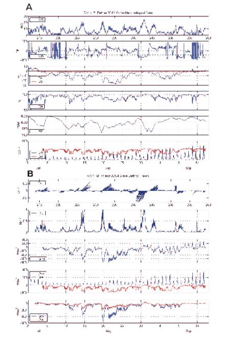 Figure 12. a) Surface meteorological measurements made during
NBP0204. The wind direction plotted is the direction the wind vector is
pointing with respect to E (e.g., a wind blowing towards the south = -90o, an eastward wind = 0o).
b) Surface wind stress and heat flux
during NBP0204. Units of wind stress are N/m2 and heat flux W/m2.
Note that these estimates are valid for OPEN WATER only.
Figure 12. a) Surface meteorological measurements made during
NBP0204. The wind direction plotted is the direction the wind vector is
pointing with respect to E (e.g., a wind blowing towards the south = -90o, an eastward wind = 0o).
b) Surface wind stress and heat flux
during NBP0204. Units of wind stress are N/m2 and heat flux W/m2.
Note that these estimates are valid for OPEN WATER only.
4.0 Nutrients (Yulia Serebrennikova, Steve Bell, Kent A. Fanning [PI not present on cruise])
In addition to temperature and salinity, dissolved inorganic nutrients (nitrate, nitrite, phosphate, ammonia, and silica) are important tracers of the circulation of waters in and around Marguerite Bay. Deeper water upwelling to shallower regions close to the peninsula should be traceable by higher nutrient signatures. Nutrient concentrations nearer to the sea surface are important to physical/chemical modeling of the fate of the plankton in the region that sustains krill, both as "targets" to be explained by nowcasting and as starting points for forecasting.
Analytical methods used for silica, phosphate, nitrite, and nitrate follow the recommendations of Gordon et al. (1993) for the WOCE WHP project. The analytical system we employ is a five-channel Technicon Autoanalyzer II upgraded with new heating baths, proportional pumps, colorimeters, improved optics, and an analog-to-digital conversion system (New Analyzer Program v. 2.40 by Labtronics, Inc.) This Technicon is designed for shipboard as well as laboratory use. Silicic acid is determined by forming the heteropoly acid of dissolved orthosilicic acid and ammonium molybdate, reducing it with stannous chloride, and then measuring its optical transmittance. Phosphate is determined by creating the phosphomolybdate heteropoly acid in much the same way as with the silica method. However, its reducing agent is dihydrazine sulfate, after which procedure its transmittance is also measured. A heating bath is required to maximize the color yield. Nitrite is determined essentially by the Bendschneider and Robinson (1952) technique in which nitrite reacts with sulfanilamide (SAN) to form a diazotized derivative that in turn reacts with a substituted ethylenediamine compound (NED) to form a rose pink azo dye which is measured colorimetrically. Nitrate is determined by difference after a separate aliquot of a sample is passed through a Cd reduction column to convert its nitrate to nitrite, followed by the measurement of the "augmented" nitrite concentration using the same method as in the nitrite analysis.
In the analytical ammonia method, ammonium reacts with alkaline phenol and hypochlorite to form indophenolblue. Sodium nitroferricyanide intensifies the blue color formed, which is then measured in a colorimeter of our nutrient-analyzer. Precipitation of calcium and magnesium hydroxides is eliminated by the addition of sodium citrate complexing reagent. A heating bath is required. Our version of this technique is based is based on modifications of published methods such as the article by F. Koroleff in Grasshoff (1976). These modifications were made at Alpkem (now Astoria-Pacific International, Inc.) and at L.Gordon's nutrient laboratory at Oregon State University.
Nitrate, nitrite, phosphate, ammonia, and silicic acid were measured from every Niskin bottle tripped from CTD casts (1125 seawater samples) on this cruise. These data are available on the cruise CDROM and will be posted to the SO GLOBEC website.
4.4 Preliminary Results for Nutrient Concentrations
The vertical hydrographic structure was near-classical with nitrate, phosphate, and silicic acid being enriched in deep water and depleted in the upper mixed layer, which is defined as the upper 50-100 meters. Nitrite and ammonium concentrations were essentially zero (i.e., less than the detection limit of the chemistry employed) in the deep water and were detectable in the mixed layer. Nutrient concentrations were uniform throughout the upper 50-100 m of the water column.
Nitrate and phosphate exhibited maxima, approximately 34 and 2.35 micromolar, respectively, at 100-200 m (Figure 13a, b). Below these depths the concentrations of both nutrients gradually decreased to 32 and 2.2 micromolar, respectively, at 1000 meters. Silicic acid concentration increased with depth from approximately 90 micromolar right below the mixed layer to 135 micromolar at 3000 m (Figure 13c). Neither deep-water nitrate nor phosphate had significant horizontal variations while deep-water silicic acid concentration was lower at off-shore locations than at on-shelf ones at the same depth. For example, 110-120 micromolar silicic acid was found in the shelf bottom water (400-500 m depth) and in the water as deep as 800-1000 m off the shelf break. These waters are believed to be the same as CDW moves onto the shelf. The intrusion of the upper layers of the CDW was characterized by low silicic acid signature and could be seen as a silica minimum at 250 m on lines 3 and 4 of the grid (Figure 13c).
The upper mixed-layer concentration ranges were 27-31, 1.9-2.2, 52-88, 0-0.21, and 0-1.2 micromolar for nitrate, phosphate, silicic acid, nitrite, and ammonium, respectively. The horizontal nutrient distribution in the upper mixed layer exhibited a considerable frontal structure. It could be aligned with the 29 micromolar nitrate contour line (Figure 14a, green contour line), which divides the study region into 3 sectors. The large central part had nitrate and phosphate concentrations less than 29 and 2.05 micromolar, respectively, and ammonium concentrations higher than 0.4 micromolar (Figure 14b). An ammonium maximum, 1.2 micromolar, occurred in the southeastern part of the grid and coincided with nitrate and phosphate minima. This ammonium maximum was lower than that of GLOBEC II (2.2 micromolar), but on GLOBEC IV, we were unable to occupy any of regions where the highest ammonium concentrations were found the previous cruises (GLOBEC I-III). The southwestern part of the grid, west of the 29 micromolar nitrate contour line, had higher nitrate and phosphate and lower ammonium concentrations than the central part, and also was characterized by higher salinity.
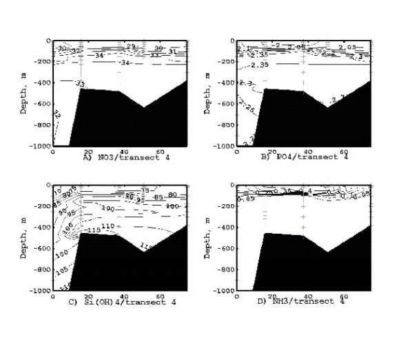 Figure 13. Vertical sections of nitrate (a), phosphate (b), silicic acid (c), and ammonium (d)
distribution on line 4 (stations 23 to 19). All concentrations are given in micromolar units.
Distance is in nautical miles from station 23.
Figure 13. Vertical sections of nitrate (a), phosphate (b), silicic acid (c), and ammonium (d)
distribution on line 4 (stations 23 to 19). All concentrations are given in micromolar units.
Distance is in nautical miles from station 23.The northeastern part of the grid along the coast of Adelaide Island had essentially zero ammonium concentration and high nitrate and phosphate concentrations, 30.5 and 2.1 micromolar, respectively (Figure 14a, b). These values were similar to those found north of Adelaide Island in Crystal Sound. These findings indicate a possible current flowing southward along the Adelaide Island coast. Also, this flow was characterized by high salinity, high silicic acid (more than 80 micromolar) and zero nitrite concentrations (Figure 14c, d).
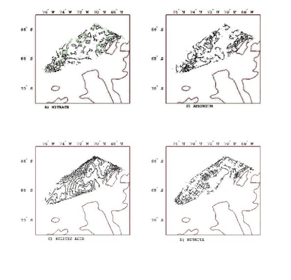 Figure 14. Horizontal distribution of nitrate (a), ammonium (b), silicic acid (c), and nitrite (d) in
the upper mixed layer. All concentrations are given in micromolar units.
Figure 14. Horizontal distribution of nitrate (a), ammonium (b), silicic acid (c), and nitrite (d) in
the upper mixed layer. All concentrations are given in micromolar units.Maximal nitrite concentrations were found in the southwestern part of the grid while the central part had moderate, 0.08-0.12 micromolar, nitrite concentrations (Figure 14d). The southwestern front lacked variations in silicic acid concentration. The central part of the grid exhibited a north-south offshore-inshore silica gradient with the lowest concentration, 52 micromolar, found at station 1, the most northern offshore location (Figure 14c). The northern region was characterized by low Si(OH)4/NO3 concentration ratios, less than 2.2, suggesting that silicic acid withdrawal was continuing in winter.
On balance, nutrient concentrations were reasonably similar to those found on the second GLOBEC cruise (NBP0104) conducted last winter in the same region.
Gordon, L.I., J.C. Jennings, Jr., A.A. Ross, and J.M. Krest, A Suggested Protocol For Continuous Flow Automated Analysis of Seawater Nutrients, in WOCE Operation Manual, WHP Office Report 90-1, WOCE Report 77 No. 68/91, 1-52, 1993.
Grasshoff, K. 1976. Methods of Seawater Analysis, Verlag Chemie, Weinheim, Germany, and New York, NY, 317 pp.
5.0 Primary Production (Karie Sines, Frank Stewart, Maria Vernet [PI not on cruise]
The objectives of the primary production component on GLOBEC IV were threefold: (1) estimation of primary productivity rates during fall and winter in the area of study; (2) understanding the mesoscale patterns of phytoplankton distribution with respect to physical, chemical and biological processes; and (3) obtaining insight into the over-wintering dynamics of phytoplankton, including their interaction with sea ice communities. Primary production was measured by the assessment of daily net production with simulated in situ experiments (SIS) and profiles with a Fast Repetition Rate Fluorometer (FRRF). The FRRF was employed with the intent of increasing resolution in the sampling of phytoplankton activity and the expectation of modeling primary production, using 14C experiments as comparison. Photosynthesis vs Irradiance experiments (PI experiments) were performed as a third method for estimating primary production and gaining information on the dynamics of light adaptation. All Photosynthesis vs Irradiance experiments were carried out on ice cores or brine samples collected by BG-235.
During this fourth Southern Oceans GLOBEC cruise, we maintained an increased emphasis on the estimation of phytoplankton biomass with measurements of chlorophyll (chla) and particulate organic carbon and nitrogen (CHN) throughout the water column. Thorough recording of photosynthetically available radiation (PAR) was carried out for the sampling duration of the cruise (surface readings and depth profiles).
5.2.1 Sampling Locations: See Table 4 for a list of the stations where the FRRF was deployed and where water for SIS experiments was collected. The FRRF was deployed at all stations where the water depth was less than 500m. At deep water stations (01, 64, and 74) a separate 100m cast was made before the main CTD cast. SIS experiments were done once a day, with water sampled from the station closest to sunrise in order to allow for accurate simulations of day lengths. Chlorophylls were sampled from all grid stations where the CTD was cast; water was filtered for CHN samples at every other station sampled along the grid.
5.2.2 Depths: Water for each SIS experiment was collected from the surface, and from depths of five, ten, fifteen, twenty and thirty meters. The FRRF was deployed as part of the CTD rosette, with a descent rate of 10 meters per minute for the upper fifty meters, 20 meters per minute to 100 meters in depth and 50 meters per minute for the remainder of the cast. Data were analyzed from the downcasts, to a depth of 150 meters. Chlorophyll and CHN were sampled at the same depths as for SIS experiments, with added collections at 50 meters, 100m, the bottom and three other intermediate depths which varied based on total cast length.
5.2.3 Equipment: Chlorophyll concentrations were measured using a Turner Designs Digital 10-AU-05 Fluorometer (serial number 5333-FXXX; calibrated using a chlorophyll a standard from Sigma Chemicals). The “Fast Track” Fast Repetition Rate Fluorometer, (serial number 182037; made by Chelsea Instruments) was outfitted with independent depth and PAR sensors. All data were recorded and stored internally; data were downloaded directly to a computer after every few casts. Samples for SIS incubations were contained in Plexiglas tubes shaded with window screening to simulate light levels. Incubations were conducted in an on-deck Plexiglas tank which was outfitted with running seawater to maintain in situ temperatures. PI curves were done in custom built incubators designed to hold 7ml vials and attached to water baths to maintain in situ temperatures. Samples were irradiated at light levels between zero and 460 μE/m2/sec. CHN samples will be analyzed upon return to the United States. Light data were collected using a Biospherical Instruments GUV Radiometer (serial number 8264) mounted on the science mast and configured with a PAR channel, as well as channels for 305, 320, 340 and 380nm wavelengths. Additional PAR data were collected using a Biospherical Instruments QSR-240 sensor (serial number 6356), also mounted on the science mast.
Over the course of forty-four science days, twenty-five SIS experiments were completed, seventeen PI curves were run on ice samples collected (from 15 different locations) by BG-235, and the FRRF was cast (with data acquired) 34 times throughout the grid.
For estimations of biomass (standing carbon stocks), both CHN and chlorophyll samples were taken; 444 CHN samples and 879 chlorophyll samples were taken from the 54 stations sampled.
Surface PAR data were collected on all days on which primary production experiments were done. GUV data were collected at one minute intervals and logged directly to computer (see Vernet Table 5 for daily measured light levels). QSR PAR data were collected as part of the JGOFS meteorological data set. Data from these last two instruments were compared to detect differences between the two types (scalar vs. cosine) of sensor (see Figure 15). PAR data were collected during each daylight CTD cast using the FRRF PAR sensor in conjunction with surface PAR data for the analysis of water column production.
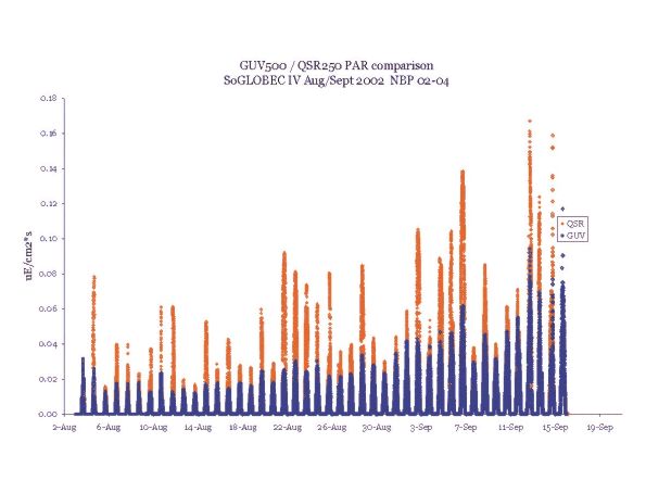 Figure 15. Plot of comparison of Biospherical Instruments QSR-240 and GUV 500 Photosynthetically Active
Radiation (400-700 nm) measurements over the course of NBP0204.
Figure 15. Plot of comparison of Biospherical Instruments QSR-240 and GUV 500 Photosynthetically Active
Radiation (400-700 nm) measurements over the course of NBP0204.Final analysis is yet to be completed on the majority of the data. Preliminary analysis suggests north-south and onshore-offshore trends in the chlorophyll levels. Similar trends were observed during GLOBECs I, II, and III. Surface chlorophyll values throughout the grid ranged from 0.02 μg/l to 0.11 μg/l, with a maximum integrated value at consecutive station 01 (7.46 μg/m2 integrated to 100m) and a minimum at consecutive station 48 (1.60 μg/m2). Water column primary production followed a pattern similar to that of chlorophyll, with highest production on the North Western corner of the grid. SIS production estimates ranged from 0.9 mgC/m2/d at station 76 to 7.2 mgC/m2/d at station 02.
Table 4: List of all primary production stations sampled.
Cons. Station # |
Latitude |
Longitude |
Data Collected |
CS7 |
66 41.68 |
67 07.50 |
FRRF |
CS4 |
66 31.73 |
67 38.15 |
FRRF |
Transit1 |
67 11.32 |
70 33.09 |
FRRF |
75 |
68 40.301 |
76 10.137 |
FRRF |
76 |
68 44.92 |
75 41.73 |
FRRF, SIS |
77 |
68 52.51 |
75 07.157 |
FRRF |
to 81 |
69 03.091 |
75 37.810 |
FRRF, SIS |
81 |
69 0.19 |
76 18.72 |
FRRF |
74 |
68 16.43 |
75 38.31 |
FRRF, SIS |
73 |
68 27.83 |
75 00.86 |
FRRF |
72 |
68 35.289 |
74 04.203 |
FRRF, SIS |
65 |
68 5.15 |
74 42.38 |
FRRF, SIS |
42 |
67 32.77 |
71 35.28 |
FRRF, SIS |
43 |
67 13.24 |
72 28.20 |
FRRF |
44 |
66 59.25 |
73 23.97 |
SIS |
46 |
67 27.516 |
73 48.004 |
FRRF |
64 |
67 31.01 |
75 5.84 |
FRRF, SIS |
48 |
67 53.65 |
72 14.19 |
FRRF, SIS |
49 |
68 4.60 |
71 36.20 |
FRRF |
40 |
68 2.00 |
70 23.96 |
SIS |
41 |
67 49.81 |
71 14.34 |
FRRF, SIS |
26 |
67 7.79 |
72 8.91 |
FRRF, SIS |
4 |
66 9.49 |
69 6.10 |
FRRF, SIS |
3 |
66 57.19 |
69 49.09 |
FRRF |
2 |
65 47.23 |
70 17.79 |
SIS |
1 |
65 37.34 |
70 36.81 |
FRRF |
13 |
66 0.45 |
71 8.71 |
SIS |
11 |
66 13.61 |
70 23.70 |
FRRF |
10 |
66 27.29 |
69 37.41 |
FRRF, SIS |
16 |
66 44.84 |
70 10.24 |
FRRF |
15 |
66 30.87 |
70 57.71 |
SIS |
23 |
66 41.13 |
71 59.77 |
SIS |
22 |
66 49.26 |
71 25.72 |
FRRF |
21 |
67 02.39 |
70 42.16 |
FRRF, SIS |
19 |
67 28.39 |
69 31.03 |
FRRF, SIS |
18 |
67 2.89 |
69 8.61 |
FRRF |
17 |
66 59.73 |
69 30.06 |
FRRF, SIS |
9 |
66 40.85 |
68 54.52 |
FRRF |
8 |
66 48.74 |
68 26.17 |
FRRF |
5 |
66 25.82 |
68 24.69 |
SIS |
RI4 |
65 7.76 |
65 30.57 |
FRRF, SIS |
RI5 |
65 7.41 |
65 30.13 |
FRRF |
Table 5: PAR (Photosynthetically Available Radiation, 400 – 700 nm) data, from BSI GUV500 mounted on Science Mast. Day lengths and daily irradiance values are calculated using PAR values above 0.0 μE/cm2*sec.
Date |
Sunrise |
Sunset |
Dec. Hours |
uE/cm² |
8/3 |
11:37 |
20:54 |
9.28 |
132.52 |
8/4 |
11:43 |
20:54 |
9.18 |
502.26 |
8/5 |
12:07 |
21:08 |
9.02 |
212.86 |
8/6 |
12:05 |
21:13 |
9.13 |
493.17 |
8/7 |
12:03 |
21:01 |
8.97 |
308.51 |
8/8 |
12:07 |
21:07 |
9.00 |
262.46 |
8/9 |
12:17 |
21:19 |
9.03 |
356.21 |
8/10 |
12:29 |
21:30 |
9.02 |
260.59 |
8/11 |
12:38 |
21:34 |
8.93 |
744.38 |
8/12 |
12:27 |
21:41 |
9.23 |
223.00 |
8/13 |
12:21 |
21:38 |
9.28 |
212.22 |
8/14 |
12:39 |
21:50 |
9.18 |
705.49 |
8/15 |
12:16 |
21:51 |
9.58 |
299.99 |
8/16 |
12:22 |
21:52 |
9.50 |
576.84 |
8/17 |
12:24 |
21:54 |
9.50 |
386.62 |
8/18 |
12:09 |
21:48 |
9.65 |
341.90 |
8/19 |
11:56 |
21:52 |
9.93 |
688.07 |
8/20 |
11:52 |
22:04 |
10.20 |
455.24 |
8/21 |
11:49 |
22:17 |
10.47 |
1658.34 |
8/22 |
11:36 |
22:24 |
10.80 |
1568.18 |
8/23 |
11:39 |
22:31 |
10.87 |
1277.77 |
8/24 |
11:32 |
22:15 |
10.72 |
637.11 |
8/25 |
11:38 |
22:11 |
10.55 |
871.46 |
8/26 |
11:24 |
22:08 |
10.73 |
561.82 |
8/27 |
11:26 |
22:11 |
10.75 |
694.04 |
8/28 |
11:15 |
22:19 |
11.07 |
1462.63 |
8/29 |
11:21 |
22:32 |
11.18 |
683.05 |
8/30 |
11:16 |
22:40 |
11.40 |
534.68 |
8/31 |
1:32 |
22:29 |
20.95 |
568.37 |
9/1 |
10:56 |
22:30 |
11.57 |
770.74 |
9/2 |
10:55 |
22:36 |
11.68 |
2116.71 |
9/3 |
10:57 |
22:36 |
11.65 |
766.91 |
9/4 |
10:44 |
22:40 |
11.93 |
1675.50 |
9/5 |
10:45 |
22:49 |
12.07 |
1669.73 |
9/6 |
10:42 |
22:48 |
12.10 |
3381.43 |
9/7 |
10:43 |
22:40 |
11.95 |
739.32 |
9/8 |
10:29 |
22:47 |
12.30 |
1682.68 |
9/9 |
10:29 |
22:47 |
12.30 |
723.52 |
9/10 |
10:20 |
22:44 |
12.40 |
1174.44 |
9/11 |
10:03 |
22:42 |
12.65 |
1253.40 |
9/12 |
10:03 |
22:51 |
12.80 |
2364.52 |
9/13 |
9:48 |
22:29 |
12.68 |
1488.08 |
9/14 |
9:48 |
22:33 |
12.75 |
1202.76 |
(Peter Wiebe, Scott Gallager, Carin Ashjian, [PI not present on cruise], Cabell Davis [PI not present on cruise])
The winter distribution and abundance of the Antarctic krill population throughout the Western Peninsula continental shelf study area are poorly known, yet this population is hypothesized to be an especially important overwintering site for krill in this geographical region of the Antarctic ecosystem. Thus, the principal objectives of this component of the program are to determine the broad-scale distribution of larval, juvenile, and adult krill throughout the study area, to relate and compare their distributions to the distributions of the other members of the zooplankton community, to contribute to relating their distributions to mesoscale and regional circulation and seasonal changes in ice cover, food availability, and predators, and to determine the small-scale distribution of larval krill in relation to physical structure of sea ice. To accomplish these objectives, the same three instrument platforms that were used on the three previous Southern Ocean GLOBEC broad-scale cruises, were used on this cruise. A 1-m MOCNESS equipped with a strobe light was used to sample the zooplankton at a selected series of stations distributed throughout the survey station grid. A towed body, BIOMAPER-II, was towyoed along the trackline between stations to collect acoustic data, video images, and environmental data between the surface and bottom in much of the survey area. An ROV was used to sample under the ice and to collect video images of krill living in association with the ice under-surface, environmental data, and current data. This section of the cruise report will detail the various methods used with each of the instrument systems or in the case of BIOMAPER-II, its sub-systems.
6.1 Zooplankton Sampling with the 1-m MOCNESS Net System
(Philip Alatalo, Peter Wiebe, Ryan Dorland, Dicky Allison, Scott Gallager, Gareth Lawson, Alec Scott)
The 1-m MOCNESS sampling of zooplankton had two main objectives. The first was to sample the vertical distribution, abundance, and population structure (size, life stage) of the plankton at selected locations across the broad-scale survey grid. The second objective was to collect information on the size distribution of the plankton, especially krill, in order to ground-truth the acoustic and video data collected using the BIOMAPER-II multi-frequency acoustic and video plankton recorder system. Using the size distribution of planktonic taxa from different depths and locations, the acoustic intensity resulting from ensonification of that water parcel will be calculated to check and ground-truth the acoustic backscatter from the BIOMAPER-II. The dominant species of the taxa enumerated using the VPR also will be identified.
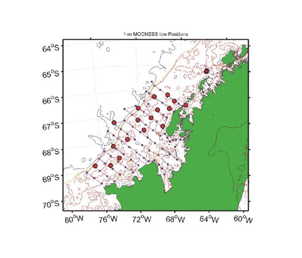 Figure 16. Location of 1-m MOCNESS tows taken on NBP0204.
 Sampling was conducted using a 1-m 2 MOCNESS (Multiple Opening/Closing Net and Environmental Sensing System) equipped with 335 µm mesh nets and temperature and conductivity probes. The MOCNESS also was equipped with a strong strobe light set to flash at 4-second intervals. Because krill are strong swimmers and likely can see slow moving nets such as the MOCNESS, the flashing strobe light was used to visually shock and to disorient krill in order to effectively capture them in the nets. For all of the tows, an Optical Plankton Counter (OPC) was mounted on the MOCNESS. Difficulty in configuring the MOCNESS and OPC was encountered at times because of interference between the two systems. The OPC sampling will be described in a separate section.
Tows were conducted at 18 locations (Table 6; Figure 16). Oblique tows were conducted from near bottom to the surface, sampling the entire water column on the down-cast. Selected depths were sampled on the up-cast with the remaining eight nets. Typically, the upper 100 m was sampled at 25 m intervals, with 50 m intervals in the intermediate depth ranges and greater intervals (150, 200 m) in the deepest depth ranges. Samples were preserved upon recovery in 4% formalin, excepting samples from the first net (oblique net haul) which were preserved in ethanol to be utilized for genetic analyses. Ctenophores were often removed prior to sample preservation for measurement and possible experimental use by Kerri Scolardi (Appendix 7).
Towing in near total sea-ice cover presents problems with regular MOCNESS deployments. Ice from the ship’s wake often can get caught underneath the towing cable, causing the net system to accelerate vertically into the bottom side of the ice. By this time the ship has often slowed to a stop and the net system then plunges down and makes contact with the bottom. This latter situation can also occur when thick ice prevents the forward motion of the ship. To avoid these problems, we carefully monitored the towing cable using pan/tilt video cameras and allowed no more cable paid out than the maximum depth of the water column. To reach the maximum depth, we had the bridge reduce the ship’s speed until the MOCNESS reached the desired depth. The wire then was hauled back at normal recovery speeds (~2 kt) to sample the remaining depths. Raising the A-frame to bring the block closer to the transom helped the cable to track closer to the stern and away from snagging ice.
Tows were conducted at 17 locations throughout the survey grid. Heavy ice prevented sampling in Marguerite Bay and nearby. A day/night comparison of zooplankton was conducted at a site near Renaud Island.
Upon return to the laboratory, plankton samples will be analyzed for displacement volume, biomass, and taxonomic and size composition. Taxonomic/size composition analysis will be accomplished using silhouette photography, yielding size specific abundance of different taxa (Large, small copepods, chaetognaths, krill, etc.) Size and abundance will then be used to extrapolate sample biomass using empirical relationships between size and taxa-specific biomass. The size/taxa information also will be used to predict the backscatter that would result from ensonification of this plankton community by the BIOMAPER-II acoustic transponders.
Table 6. Summary of 1-m MOCNESS Tows (local Date/Time)
TOW |
STATION |
DATE |
TIME |
LATITUDE (S) |
LONGITUDE (W) |
1 |
CS |
7-Aug-02 |
13:46 |
66 31.7 |
67 19.2 |
2 |
77 |
12-Aug-02 |
20:42 |
68 50.7 |
75 6.7 |
3 |
82 |
14-Aug-02 |
3:35 |
68 48.3 |
76 46.2 |
4 |
72 |
16-Aug-02 |
0:35 |
68 34.6 |
74 7.1 |
5 |
65 |
17-Aug-02 |
12:42 |
68 6.3 |
74 41.5 |
6 |
42 |
19-Aug-02 |
10:28 |
67 31.4 |
71 26.7 |
7 |
45 |
22-Aug-02 |
2:02 |
67 11.2 |
74 27.2 |
8 |
62-48 |
24-Aug-02 |
19:20 |
67 52.2 |
73 09.9 |
9 |
26 |
29-Aug-02 |
10:10 |
67 07.8 |
72 03.1 |
10 |
4 |
1-Sep-02 |
7:04 |
66 9.2 |
69 6.6 |
11 |
11 |
3-Sep-02 |
18:30 |
66 13.5 |
70 23.6 |
12 |
16 |
4-Sep-02 |
20:25 |
66 44.5 |
70 9.9 |
13 |
23 |
6-Sep-02 |
5:55 |
66 40.3 |
71 57.7 |
14 |
21 -20 |
7-Sep-02 |
4:15 |
67 03.2 |
70 43.3 |
15 |
19 |
8-Sep-02 |
0:22 |
67 22.5 |
69 33.0 |
16 |
9 |
9-Sep-02 |
10:09 |
66 44.2 |
68 54.3 |
17 |
5 |
10-Sep-02 |
4:04 |
66 25.9 |
68 30.6 |
18 |
RI1 |
11-Sep-02 |
6:45 |
65 11.0 |
65 33.9 |
19 |
RI3 |
11-Sep-02 |
19:15 |
65 8.8 |
65 31.7 |
Abundance of krill appeared to have increased since the fall cruise earlier this year. This was confirmed by acoustic backscatter seen from the Simrad EK500, ADCP, and BIOMAPER-II. While the presence of krill increased as we steamed northward, only along the mid to outer shelf were krill frequently abundant. Ice prevented sampling in all of inner and outer Marguerite Bay. Heavy krill biomass (Euphausia superba) was observed at Crystal Sound and north next to Renaud Island, consistent with high abundance reported northwest of the Peninsula These densities of krill were comparable to those obtained in Crystal Sound and Matha Strait on our fall cruise of 2001, NBP0103. Thysanoessa macrura was the most numerous of the euphausiids, often found throughout the water column between 200-0m, while E. superba was more often distributed in shallow, distinct layers or patches between 100-0m. E. crystallorophias and E. tricantha were rare and occurred between 350-200 m.
Copepods formed the deep scattering layers below 200 m. These layers were often comprised of large calanoid copepods such as Calanus propinquus residing below smaller calanoid and oithonid copepods. Especially in the northern sector of the sample grid, krill appeared to displace copepods at least in terms of biomass. This was especially evident at the 24-h station at Renaud Island. Copepods were dominant between 500-350 m in the daytime and virtually absent at all depths in the evening sample. T. macrura was present at mid-depth during the day, with E. superba very abundant between 50-25 m. This layer rose to 25-0 m during the evening and was extremely abundant.
To what extent pteropods, ostracods, radiolarians, and gelatinous organisms contributed to the scattering layer is unclear. At various stations, these organisms reached high densities, but usually contributed evenly to the overall biomass for nearly every tow. Chaetognaths, in particular were very numerous at nearly all depths. Oddly, the Video Plankton Recorder mounted on BIOMAPER-II made few visual observations of chaetognaths. Observations of fish larvae by the SeaRover ROV were confirmed by frequent catches in surface nets by MOCNESS especially in the southern part of the survey grid. Pteropods, primarily Limacina sp. and their gymnosome predators, Clione sp. increased in abundance dramatically as we sampled north and east. These mollusks may indicate the presence of the East Wind Drift Current moving along the coast. With the exception of high-krill stations, overall biomass present above 100 m was low.
Special thanks to ET’s Fred Stuart and Todd Johnson, MT’s Nancy Ford, Jamee Johnson, and Stian Alesandrini, and the bridge (Cap’t Joe, Val, Mike, Paul, and Rachelle) for operations, to Ryan Dorland for flying the net system, and to Kendra Daly, Joe Donnelly, and Tom Bailey for help in identification.
The overall goal of our group is to quantify the horizontal and vertical distribution of adult and larval krill and other zooplankton taxa, using as our primary tool the BIO-Optical Multi-frequency Acoustical and Physical Environmental Recorder or BIOMAPER-II. BIOMAPER-II is a towed system capable of conducting quantitative surveys of the spatial distribution of coastal and oceanic plankton/nekton. The system consists of a multi-frequency sonar, a video plankton recorder system (VPR), and an environmental sensor package (CTD, fluorometer, transmissometer). The acoustic system collects backscatter data from a total of ten echosounders (five pairs of transducers with center frequencies of 43 kHz, 120 kHz, 200 kHz, 420 kHz, and 1 MHz), half of which are mounted on the top of the tow-body looking upward, while the other half look downward. This arrangement enables acoustic scattering data to be collected for much of the water column. The VPR is an underwater video microscope that images and identifies plankton and seston in the size range 0.5-25 mm and quantifies their abundances, often in real time.
Together, the acoustic and VPR systems allow high-resolution data to be obtained on adult and larval krill and their prey. The acoustic data provide distributional information at a higher horizontal resolution than is possible with the VPR, while the video data provide taxa-specific abundance patterns along the towpath of the BIOMAPER-II. The VPR also allows for direct identification, enumeration, and sizing of objects observed in acoustic scattering layers, such that the VPR data are used to ground-truth the acoustical data.
Also included in the system are an electro-optic tow cable, a winch with slip rings, and van which holds the electronic equipment for real-time data processing and analysis. The towbody is capable of operating to a depth of 500 meters at 4 to 6 knots. The system can be operated in a surface towed down-looking mode, in a vertical oscillatory "towyo" mode, or in a sub-surface up/down looking horizontal mode. All three modes were used to varying extents on NBP0204. To enhance the performance and utility of BIOMAPER-II in high sea states, the system also includes a winch, slack tensioner, over-boarding sheave/docking assembly, and hydraulic power pack. The slack tensioner is designed to decouple the towbody from the movement of the ship and was not used during NBP0204 since the presence of thick ice kept vessel movement to a minimum. The power pack, which on earlier cruises had been located in the aft cargo hold, was moved to a small heated van located on the port side of the deck next to the winch. This had to be done because of the construction of a through-hull well that passed through the area of the cargo hold where the power pack historically had been installed.
As on the first three SO GLOBEC broad-scale cruises (NBP0103, NBP0104, NBP0202), BIOMAPER-II was deployed from the stern of the RVIB N. B. Palmer. Attached to the starboard side of the A-frame on the Palmer was a stiff arm, designed and constructed at WHOI, to lower the over-boarding sheave/docking assembly to a level that would minimize the distance that BIOMAPER-II needed to be hauled up to be docked and still clear the stern rail when the A-frame was boomed in. The stiff arm was modified between NBP0202 and NBP0204 to reduce the width and thus enable the pad-eyes on the center and port side of the A-frame to be used for sheaves to tow the Tucker Trawl and 10-m MOCNESS. It was shackled at two points to pad eyes on the top of the A-frame. The over-boarding sheave articulated and was equipped with a hydraulic ram, so that its position could be adjusted to keep the docking mechanism vertical during launch and recovery, and to move it inboard of the wire when towing.
An electro-optical cable with a diameter of 0.68 “ was used to tow BIOMAPER-II. The tow cable contained three single mode optical fibers and three copper power conductors. Data telemetry occupies one fiber (using two colors), the video the second, and raw acoustic data the third. A cable termination matched to meet the strengths of the towing cable and the towed body's towing bail was designed and built at WHOI.
In anticipation of the high winds, cold temperatures, and wet working conditions on the stern deck of the Palmer, a shipping container, modified into a working “garage” for BIOMAPER-II, was located on the starboard side of the vessel centerline and forward of the small stern crane. The towed body was easily moved on dollies to a position where it could be picked up by a motor drive hoist suspended from a movable I-beam and moved inside the van. The van again proved essential when working on the towed body for maintenance, repair, or dry warm storage.
The BIOMAPER-II control van was located on the 03 level inside the helicopter hanger. The heated van accommodates three or four individuals and computers for four operations: acoustic data acquisition and processing, VPR data acquisition and processing, ESS acquisition, and hardware monitoring. A power supply in the van provides BIOMAPER-II with 260 volts of DC power. A VHF radio base station and two portable units provided communication with the bridge, deck, and labs. Two video cameras were mounted on an aluminum mast attached to a corner post of the small van with the power pack and had monitor outputs in the control van. One, a fixed camera, was used when towyoing BIOMAPER-II for observing the winch. The second, with pan, tilt, zoom, and focus controls, was for observing the slack tensioner and the overboarding sheave during launch and recovery of the towed body. A third camera (also pan and tilt) was installed on a post about mid-ships on the helicopter pad. This camera was used for observing the cables towing BIOMAPER-II and the MOCNESSs and for early detection of sea ice snagging the cables. This latter camera had outputs to all of the ships monitors. Inputs to the van from the Palmer’s navigation and bathymetry logging system, included P-code GPS (9600 baud), Ashtech GPS (4800 baud), and Bathy bottom depth information. In addition, there was an ethernet connection in the van to the ship’s network.
For the most part, the system performed well under all conditions experienced during the cruise. Unlike during the 2001 winter cruise, the BIOMAPER-II suffered no structural damage due to collision with ice or the stern of the vessel. On two occasions when the ship was repeatedly backing and ramming, the electro-optical towing wire became frayed. Although we were able to repair these frays and did not have to re-terminate, for the sake of caution we did not pay out wire from the winch beyond the repaired frays. This reduced our operational depth first from 500 to 200 m, and later to 150 m.
In order to collect the best data possible, the towbody should remain perfectly level while being towed, but during many of the early tows of NBP0204, it was flying at as much as a 22 degree angle nose-upward and 22 degrees to port. Initial attempts at solving this problem involved angling the adjustable aileron on the tail fin slightly downwards and adding horizontal stabilizers mid-way up the fin. Since these measures failed to solve the problem, the plastic tail fin used since the start of the cruise was replaced by a plywood one made last winter. The plastic fin had a strong curve to starboard, whereas the woods one was much straighter. Making the replacement brought the pitch and roll down to reasonable levels.
Overall, the VPR system encountered very few problems. During one tow the strobe lens fell off, causing the strobe to come out of alignment, but this problem was easily remedied. Similarly, the Environmental Sensing System (ESS) suffered no difficulties, other than occasional minor ground faults due to leaking connectors. In contrast, between August 5 and August 16, the acoustic system suffered multiple setbacks. First, the two highest frequency transducers (420 and 1000 kHz) spontaneously ceased transmitting. Long hours of trouble-shooting, led by Scott Gallager and Alec Scott, eventually traced the problem to a set of blown power mosfets on the high frequency transmit board. On August 11, two days after replacing these mosfets and repairing the system, the 43 kHz transducers also spontaneously ceased to transmit. Before this new problem was fully addressed, transmission ceased or became severely weakened on all transducers. A further 40 hours of trouble-shooting identified three problems: a burned-out resistor on the high frequency transmit board, a mal-functioning chip on the 43 kHz receiver board, and an as-yet-unidentified malfunction in the multiplexor board. This last problem was fixed by simply replacing the multiplexor board with a spare that was on board, which restored proper functioning at 120 and 200 kHz. By this point, the BIOMAPER-II group had missed a fair amount of the survey. Rather than risk losing even more survey time, the decision was made to complete the remainder of the cruise with only these two frequencies and to not spend additional time repairing the other frequencies.
A listing of BIOMAPAR-iII deployments and the data files and tapes recorded during the cruise are provided in Appendix 8.
6.2.1 Acoustics Data Collection, Processing, and Results
(Gareth Lawson, Peter Wiebe, Carin Ashjian [not present on Cruise], Scott Gallager, Cabell Davis [not present on Cruise])
The use of high-frequency sound to ensonify the water column and produce echograms that portray the vertical distribution of entities that backscatter sound is one of the few means of visualizing their continuous distribution and gaining some sense of their abundance. Single frequency systems while useful in this regard, are much less capable of providing insight into the taxonomic makeup of the scatterers than is a system with multiple frequencies. Likewise, echo integration provides an estimate of the strength of the backscattering as a function of depth, but does not provide any information about the size range of the entities whose backscattering has been integrated. The echosounder on BIOMAPER-II provides both echo integration data and target strength data on four of the five pairs of transducers and as a result, in combination with the ground-truthing data obtained with the 1-m MOCNESS and the VPR, should be able to provide considerable information about the distribution and abundance of the zooplankton populations along the survey tracklines. On NBP0204, a large quantity of acoustic data were collected during the six weeks of the survey, in spite of the down time for repairing the towed body. Approximately 300 GB of raw acoustic data were recorded and much of these data were processed in real-time so that echograms could be created and comparisons made of the changes in the backscattering fields as the cruise progressed. Refinements to the processed data are required before a final analysis can be done, but a preliminary look at the data presented below provides insight into the patterns that were observed and the changes that took place between previous cruises and this fourth SO GLOBEC broad-scale cruise.
BIOMAPER-II collects acoustic backscatter echo integration data from a total of ten echosounders (five pairs of transducers with center frequencies of 43 kHz, 120 kHz, 200 kHz, 420 kHz, and 1 MHz). Due to differences in absorption of acoustic energy by seawater, the range limits of the transducers are different. The lower frequencies (43 and 120 kHz) collect data up to 300 m away from the instrument (in 1.5 m range bins), while the higher frequencies (all with 1 m range bins) have range limits of (150, 100, and 35 m respectively).
There were three transducer configurations used on this cruise. The original (and standard) configuration and MUX assignments were used for only a very few days until the problems described above developed with the upper frequencies. The second configuration involved only the 120 and 200 kHz transducers, both with their standard MUX assignments. Finally, in order to test whether MUX assignment had any impact on the difference in scattering levels observed between the up- and down-looking 120 kHz transducers, our final configuration had the positions of the up- and down-looking 120 kHz transducers switched.
The acoustic data were recorded by HTI software and stored as .INT, .BOT and .RAW files on a computer hard drive. The data were archived on removable 40 gig hard drives. The .INT and .BOT files were further post-processed using a series of Matlab files (written by Joe Warren, Andy Pershing, Gareth Lawson, and Peter Wiebe) to combine the information from the upward and downward looking transducers. The acoustic backscatter data from the HTI system were then integrated with environmental data from the ESS onboard BIOMAPER-II. These latter data included depth of the towed body, salinity, temperature, fluorescence, transmittance, and other parameters. The integrated acoustic and environmental data were concatenated into typically half-day (am or pm) chunks and used to make maps of acoustic backscatter throughout the entire water column (or at least to the range limits of the transducers). In addition, information about the three-dimensional position of BIOMAPER-II (pitch, roll, yaw) and data from the winch (tension, wire out, wire speed) were recorded.
The .INT data format described above is the standard HTI output file format, which averages the acoustic data over four ping intervals. This is done to reduce file size, but has the unfortunate consequence of also reducing the horizontal resolution of the data. On this survey, ping-by-ping acoustic data were also recorded, using new beta-release software provided by HTI. This cruise marks the first time our research group has collected acoustic data in this format. As such, we are still in the process of developing Matlab code for processing and analyzing these data. Once this development and subsequent analyses are completed, the ping-by-ping data will undoubtedly provide very useful information on resolution-dependent questions such as patch structure.
In this report, analysis of the acoustic data collected with BIOMAPER-II is limited to qualitative descriptions of overall patterns. Future quantitative analyses and examinations of the distributions of particular taxa will await the incorporation of the acoustic data with information derived from MOCNESS net tows and the video plankton recorder (VPR).
Due to ice conditions, survey coverage was lower than for all three previous SO GLOBEC cruises. As on previous surveys, the general pattern of backscattering across most of the survey area involved low backscattering in the surface mixed layer, moderate backscattering in the pycnocline, a midwater zone that typically had faint scattering, and when the bottom was within range of our transducers, a well-developed bottom scattering layer extending 40 to 100 m above the bottom (Figures 17a, b). Less regular was the appearance of dense patches of variable size at depths ranging from the surface to 350 m. Overall, backscattering levels were substantially reduced from the fall cruise, and were comparable to those observed in last year’s winter cruise. Ground-truthing the specific composition of the patches and layers observed acoustically will be made possible as the MOCNESS and other net tow samples are processed, as well as the VPR images examined.
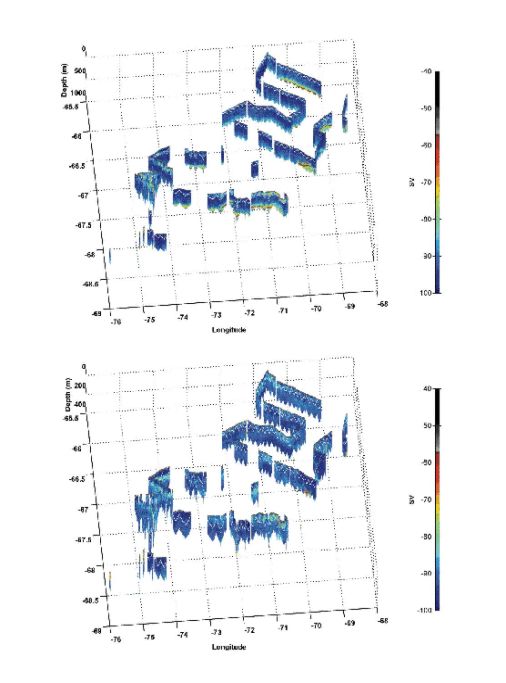 Figure 17. a) Volume backscattering data
collected during the NBP0204 broad-scale survey with BIOMAPER-II at 120 kHz. The black/red region at the top of
the echograms shows high backscattering due to the wake of the ship. The white
line indicates the position of BIOMAPER-II as it was towyoed along the survey
transects. b) Volume backscattering data collected during the NBP0204 broad-scale
survey with BIOMAPER-II at 200 kHz.
Figure 17. a) Volume backscattering data
collected during the NBP0204 broad-scale survey with BIOMAPER-II at 120 kHz. The black/red region at the top of
the echograms shows high backscattering due to the wake of the ship. The white
line indicates the position of BIOMAPER-II as it was towyoed along the survey
transects. b) Volume backscattering data collected during the NBP0204 broad-scale
survey with BIOMAPER-II at 200 kHz.Krill-like scattering was observed at numerous locations within the survey area, and came in three general forms. At the southernmost reaches of the surveyed area (near stations 72, 76, and 77), as well as at the mouth of Marguerite Bay (stations 49 and 40), large layers of scattering 80 to 100 m tall and up to 8 km long were found in the mixed layer, reaching backscatter levels of -54 dB. On those occasions when the BIOMAPER-II passed through one of these layers, adult krill often were observed. At other locations in the survey grid, particularly in the northwestern sector of the grid, more discrete patches of dense (up to -52 dB) krill-like scattering were observed. These patches were often tall (10 to 45 m) and narrow (35 to 150 m), and were generally found within the mixed layer (20 to 100 m depth). VPR observations made when the BIOMAPER-II intercepted one of these shallow patches again indicated the presence of adult krill. Finally, a number of discrete and large (50 to 125 m tall and mostly 150 to 800 m long) patches of backscattering were observed at depths below the mixed layer (100 to 350 m). These patches were very dense (up to -50 dB) and particularly abundant at the outer edge of the continental shelf in the central sector of the survey grid and in close to shore near Adelaide Island. In this latter region, as the bottom became shallower near Johnston Passage (station 19), we observed a series of patches near the bottom that were the largest of the cruise, reaching 3360 m in length. Due to their deep distribution, no VPR observations were made of any of these deep patches. On at least two occasions, however, the MOCNESS sampled a patch and captured large krill. The presence of both the shallow and deep krill-like patches at the edge of the shelf is particularly interesting since few patches attributable to krill were present in such areas during the last winter cruise.
Another feature that has occurred frequently on this and the three previous cruises was the presence of a shallow zone of weak backscattering above the pycnocline. During NBP0204, some sort of shallow scattering layer was present throughout almost the entire survey grid, and often more than one layer was evident. Off the continental shelf and near the shelf break in the central and northern sectors of the survey grid, a tall (50 to 80 m) layer of weak backscattering (-80 to -70 dB) was evident in the mixed layer, often most dense just at the top of the pycnocline. VPR observations suggested that this layer generally was composed of dispersed krill (juvenile and larval stages in particular), copepods (including large calanoids), diatom chains, radiolarians, and occasional pteropods. Often very thin layers were also present, 1 to 3 m in vertical extent and again associated with the pycnocline. In some locations, these thin layers were the only shallow scattering features in evidence. Profiles of the water column made with the CTD-Microstructure Profiling System (CMiPS) concurrent with acoustic observations by the BIOMAPER-II suggest a potential association between these thin layers of backscatter with regions in the water column of particular kinds of microstructure (Figure 18a). Sharp density gradients in the water column, such as at the pycnocline or within microstructure layers, can reflect appreciable amounts of sound. The observed thin acoustic layers therefore may stem from sound scattered by physical features of the water column itself, by organisms associated with these features, or some combination of these physical and biological sources. Distinguishing among these possibilities is one of the ongoing goals of the BIOMAPER-II research group.
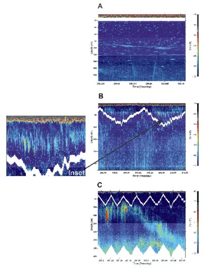
Figure 18. a) Acoustic observations made at 120 kHz on September 7, 2002 (YD 250) concurrent to CTD-Microstructure Profiling System (CMiPS) casts at station 20. The vessel was stationary during the period of observation. The diagonal lines below 100 m in the middle of the echogram trace the path of the CTD cast. On the CMiPS downcast, a region of abrupt temperature change (0.5 degrees Celsius) was observed at 93 m, coincident with the scattering layer observed acoustically. b) Possible vertical circulation cells observed at 120 kHz on September 3, 2002 (YD 246) while towing from station 12 to station 11. Inset is a zoomed-in view of the right-hand side of the echogram, showing the regularity in spacing of bands of high and low backscatter. c) Diel vertical migration of a zooplankton scattering layer observed while towing between stations 19 and 18 on September 8, 2002 (YD 251). The white line indicates the path of the BIOMAPER-II as it was towyoed along the survey line.
In the northern sector of the survey grid, the shallow scattering layer showed enhancements in backscattering intensity at fairly regular intervals (Figure 18b). These enhancements were not present throughout the layer, but when evident, were spaced approximately 200 m apart. The regularity in the alternation between these areas of high and low scattering suggests the possible presence of vertical circulation cells: vertical current structures that serve to concentrate planktonic organisms (and hence backscatter) in distinct vertical bands. When seawater freezes it leaves behind its dissolved salts, in a process called brine rejection. This results in denser water at the sea surface than deeper in the water column, leading to downwards movement of surface waters and the formation of circular current ‘cells.’ Such a process could be at play in this region. Similar features were observed near the shelf break along transect 6 during the NBP0104 winter cruise. On one instance while towing between stations 1 and 13, the shallow scattering layer (and a deeper layer) showed wave-like oscillations in depth, suggesting the possible presence of an internal wave. This station was very close to the continental shelf break, and internal waves often form at and propagate away from shelf breaks.
In addition, some evidence of diel vertical migration by the zooplankton populations was observed (Figure 18c). In the early morning of September 8, for example, a layer of high backscattering was present near the base of the pycnocline, at 80 m. At 0630 this layer began to descend deeper in the water column, and by 0845 had reached a depth of 350 m: a clear case of a diurnal vertical migration, occurring at a rate of 1.5 m/min.
Throughout the entire surveyed area, nearly every time the bottom came within range of our transducers, a distinct bottom layer was present. The only time such a layer was not observed was near station 8, at a point when the bottom was only 150 m deep and dropping off rapidly. The bottom layer was visible at both 120 and 200 kHz, although it was seen best on the 120 kHz because of its greater range. The exact nature of the layer was quite variable. At times, only single layer was evident, generally of fairly uniform density. On other occasions, two adjacent layers of different structure were present: a weak scattering layer extending from the bottom to 40 to 100 m above bottom, followed by a layer of more sparsely distributed large individual targets extending up an additional 50 m. On August 20, BIOMAPER-II was towed along transect 6, and a single bottom layer was present. As the vessel approached the continental shelf break, and also as it got dark, the top-most reaches of this layer coalesced into more sparsely distributed patches and groups of stronger targets. Whether this change from one to two bottom layers represented a diurnal change in the aggregative behavior of organisms at these depths or an along-transect change in the near-bottom species composition remains to be determined, but poses an intriguing question. MOCNESS tows through these bottom layers sampled many copepods, large krill (Thysanoessa spp. and Euphausia tricantha), myctophid fishes, and large chaetognaths. The persistent occurrence of a bottom layer was a feature also observed on the previous three cruises. It is noteworthy that unlike the present cruise, during the fall 2002 survey, a pronounced bottom layer was not present on the outer shelf.
Four in situ calibrations of the acoustic system were undertaken over the course of the cruise. To do the calibrations, the upper looking transducers were taken out of their top frame mounts and bolted into a calibration rig, so that both sets of transducers were side by side facing downward. A series of four standard targets (two calibration balls of diameter 31.8 mm, one of diameter 21.2 mm, and a ping pong ball) were suspended underneath the transducers at 5, 6, 7, and 8 m. For an ideal calibration, the balls should be positioned exactly in the center of the acoustic beam, at least 5 m from the transducer. In the first two calibrations, we experienced substantial difficulties in positioning the ball appropriately, and only low quality data were collected. During the final two calibrations, however, we were able to position the ball properly, and obtained high quality data for the 120 and 200 kHz transducers. More detailed analyses of these calibration data will be critical to scaling measurements of acoustic backscattering to quantitative estimates of zooplankton abundance.
6.2.2 Video Plankton Recorder (S. Gallager, C. Ashjian [PI not present on cruise], C. Davis [PI not present on cruise])
The Video Plankton Recorder (VPR) is an underwater video microscope that images and identifies plankton and seston in the size range 0.5–25 mm and quantifies their abundances, often in real time. As part of the Southern Ocean GLOBEC Program, the goal of the VPR studies is to quantify the abundance of larval krill as well as krill prey, including copepods, large phytoplankton, and marine snow.
6.2.2.2.1 Cameras and strobe: A two-camera VPR was mounted on the BIOMAPER-II towed body for this cruise. The cameras and strobe were mounted on top of BIOMAPER-II, forward of the tow point. The cameras were synchronized at 60 HZ with a 16-watt strobe.
6.2.2.2.2 Calibration: The two cameras were calibrated to determine the field of views (width and height of the video field) of the imaged volumes for each camera by using a translucent grid placed at the center of focus. The field width and height of the high magnification camera were 11 x 9 mm, respectively, while the low magnification camera had a field of view of 16.5 mm x 13 mm. The depth of field of the imaged volume was estimated to be 50 mm for the low magnification camera and 55 mm for the high magnification camera. The depth of field can be quantified by videotaping a tethered copepod as it is moved into and out of focus along the camera-strobe axis using a micropositioner, while recording (on audio track) the distance traveled by the copepod in mm. The cameras and strobe will be shipped back to Woods Hole after the cruise in their final configuration for final calibration and the establishment of the depth of field.
6.2.2.2.3 Video Recording and Processing. The analog video signals (NTSC) from the two cameras were sent from the fiber optic modulator (receiver) in the winch drum through coaxial slip rings and a deck cable to the BIOMAPER-II van. The incoming video was stamped with VITC and LTC time code using a Horita Inc. model GPS time code generator. Horita character inserters were used to burn time code directly on the visible portion of the video near the bottom of the screen. The two video streams with time code then were recorded on two Panasonic AG1980 SVHS recorders and looped through these recorders to two image processing computers.
The software package Visual Plankton (WHOI developed and licensed) was used to process the VPR video streams. This software is a combination of Matlab and C++ code and consists of several components including focus detection, manual sorting of a training set of in-focus images, neural net training, image feature extraction, and classification. Visual Plankton was run on two Dell Inc. Pentium 4 1.4GHZ computers (Windows 2000 operating system) containing Matrox Inc. Meteor II NTSC video capture cards. The two video streams (=camera outputs) were processed simultaneously using the two computers (one stream per computer).
Regions Of Interest (ROI) were extracted and saved to “tif” files following a focus detection program written in C++. This step was conducted in real time as the video images were collected. The focus detection program interfaces with the Matrox Meteor II board using calls to the Mil-Lite software written by Matrox Inc. The incoming analog video stream first was digitized by the Meteor II frame grabber at field rates (i.e. 60 fields per second). Each field was digitized at 640 by 207 pixels, cropping out the lower portion of the field to remove the burned-in time code. The digitized image then was normalized for brightness and segmented (binarized) at a threshold (150) so that the pixels above the threshold were set to 255 and ones below the threshold were set to 0. The program then ran a connectivity routine that stepped through each scan line of the video field to determine which of the “on” pixels (those having a value of 255) in the field were connected to each other. Once these clusters, termed “blobs”, were found, it was determined whether they were above the minimum size threshold, and if so, they were sent to the edge detection routine to determine the mean Sobel edge value of the blob. On previous cruises, if the Sobel value was above some focus threshold, the region of interest (ROI) containing the blob was expanded by a specified constant and saved to the hard disk as a TIFF image using the time of capture as the name of the file. On the present cruise, every ROI was saved, irrespective of Sobel-determined focus. The digitized video, as well as the segmented image, Sobel sub-images, and final ROIs were all displayed on the computer monitor as processing took place. ROI files were saved in hourly subdirectories contained in Julian day directories.
Once a sufficient number of ROIs were written to hourly directories, a subset of the ROIs was copied to another directory for manual sorting of the images into taxa-specific folders using an image-sorting program (Compupic). Another program was run to extract the features and sizes from these sorted ROIs and set up the necessary files for training the neural network classifier.
6.2.2.2.4 Plankton Abundance and Environmental Data
Plankton abundances coincident with the environmental data (e.g., pressure, temperature, fluorescence) are obtained by binning the times when specific plankton were observed into the time bins (4-second intervals) of the navigational and physical data from the environmental sensors. The number of animals observed during each 4-second interval is divided by the volume imaged during that period to produce a concentration of individuals/L at that time/depth. Size parameters for each individual and the mean size of individuals within each time interval are derived from parameters defined during the feature extraction procedure; area is used to describe particle size since it is relatively independent of orientation, unlike length, and can easily be converted to equivalent spherical diameter for comparison with other plankton size quantification instruments. These data are combined to produce comprehensive files of the environmental, plankton abundance, and plankton size data which then were utilized to produce curtain plots of environmental parameters (data mapped to a regular grid using the NCAR ZGRID routine) and dot plots or curtain plots of the plankton abundances. Note that plankton abundances were not calculated during the cruise itself, but will be calculated later at WHOI. Plots of the environmental variables were produced in real time during the cruise.
Video Plankton Recorder data were collected along the survey grid between CTD stations as the BIOMAPER-II was towyoed between depths of 20-30 m and the maximum operating depth, or to within what was deemed a safe distance from the bottom and the under-ice surface. As described above (see section 4.2), the maximum operating depth changed from 500 to 200 to 150 m over the course of the cruise, due to fraying of the tow cable. When in ice, the upper depths of the sampling range (30 m) were somewhat deeper than usually used with the BIOMAPER-II in order to avoid collisions between ice chunks and the vehicle. The ship steamed at 5 knots during the grid sampling.
Sampling in an ice-covered sea produces multiple challenges, the most notable being the dangers associated with snagging the cable on ice floes in the wake of the ship, and the ship coming to a halt to back and ram because of heavy ice conditions. Fortunately, the ice encountered during most of the cruise could be traversed easily by the ship with ice chunks advected away from the wake and clear of the wire. The wire position was monitored closely using a dedicated video camera at all times when the ship was in ice. In conditions of very thick ice, it was necessary to recover the BIOMAPER-II so that the ship could more easily maneuver. Much VPR survey time was lost early in the cruise due to the BIOMAPER-II being on board while the acoustic system was repaired.
6.2.2.3 VPR Preliminary Results
The quality of the video signals from both cameras was very high during the entire cruise. A large number of images was collected from both cameras, resulting in a storage problem. The number of ROIs easily overwhelmed the storage space available on the ROI collection computers. Diligent backups of ROIs during the cruise permitted us to delete already backed up tows to make room for new images from subsequent tows. Because the BIOMAPER-II was in use for much of the cruise, and hence the computers were busy, it was difficult to accomplish much beyond disk space management during the cruise.
Images were transferred from the primary ROI collection computers to an additional computer for identification. For all of the BIOMAPER-II tows when VPR data were collected, images from the high magnification camera that could be definitively identified through visual scrutiny as krill, copepods, marine snow, diatom chains, or radiolarians were set aside for future use in developing classification algorithms. Remaining images were categorized as ‘out of focus’ or ‘other.’ Development of classification algorithms did not take place during the cruise, and will await further analysis of the VPR data at WHOI.
Since classification algorithms were not generated during the cruise, quantitative estimates of the abundances of particular taxa are not yet available. For the purposes of this report, analyses of the VPR data therefore are restricted to qualitative descriptions of overall patterns. In general, plankton abundances appeared to be low. The cameras on the VPR have an image volume of approximately 1.6 ml for the high magnification camera and 20 ml for the low magnification camera. The imaging rate is 60 images per second, giving volumes sampled of 6 liters per minute and 72 liters per minute, respectively. As such, for us to catch an image of a planktonic organism they must be relatively abundant, typically greater than about 20 per cubic meter. Such densities were quite rare during NBP0204 compared with previous cruises. Unfortunately, beyond this general observation, it is presently not possible to make quantitative comparisons between this and earlier cruises.
Images captured on both cameras in the 0 to 100 m depth range suggest that the mixed layer planktonic community was composed primarily of copepods, krill, diatoms (single cells and chains), and radiolarians. Observations of ostracods, ctenophores, thecosomatous pteropods, and larvaceans were also common. Less frequently observed taxa included foraminifera, chaetognaths, tomopterid worms, and medusae. Many copepods were further identified to the genera Calanus and Oithona. As on previous cruises, the presence or absence of a bi-lobed eye frequently made it possible to classify krill as Euphausia or Thysanoessa. Numerous diatom chains were observed during the cruise, but in contrast to the fall cruise, virtually no algal mats were evident. Images captured by the VPR commonly were associated with weak scattering layers observed acoustically and as such, were frequently clustered around the pycnocline (see section 6.2.1.3). In general, mixed layer community structure appeared to be quite consistent throughout the survey area.
On two occasions, there was distinct evidence of a layer of ctenophores immediately below the mixed layer community. On August 26 (YD 238), at 0600 local time the ship was traveling through an open lead between stations 49 and 40. The VPR observed a dense layer of krill between 65 and 20 m with another dense layer of copepods between 20 m and the surface. Below the krill layer was a third layer extending between 107 and 65 m and consisting of ctenophores, copepods, and notably, Beroe, a large predatory lobate ctenophore. A similar layer of ctenophores was observed immediately below a mixed layer composed of krill and diatoms on Sept 3 (YD 246), between stations 12 and 11.
In terms of their association with concurrently-collected acoustic data, observations of krill were of three sorts. On numerous occasions the BIOMAPER-II intercepted a dense acoustic patch and large (likely adult) krill were observed on one or both cameras. At other times, images of krill typically smaller than 1 cm (i.e., furcilia or other larval stages) were captured when diffuse shallow scattering layers were observed acoustically; frequently these krill were associated with thinner and denser sub-layers within the overall acoustic layer. At still other times, virtually no acoustic scattering was evident, but individual krill were observed by the VPR. Such diffuse krill were observed as deep as 160 m.
Below the mixed layer, the VPR captured images of a diverse species assemblage, including copepods, krill, gelatinous zooplankton (e.g., Medusae), worms, and radiolarians. The ability of the VPR to sample these deep regions was severely compromised as of August 24, when the tow cable became frayed and the maximum operating depth of the BIOMAPER-II was reduced to 150 m.
6.2.3 Water column hydrographic and environmental characteristics
6.3 ROV observations of larval krill distribution, abundance, and behavior under-ice
(Scott Gallager, Philip Alatalo, and Alec Scott)
The objective of the ROV studies is to observe and quantify the distribution, abundance, behavior and size distribution of larval krill in association with the underside ice surface and sea surface hydrography. The WHOI SeaRover was equipped with a variety of physical and biological sensors including a stereo camera system with a field of view of 0.5 m3, a synchronized strobe, a CTD, an Imagenix 881a 630 kHz-1 MHz sector scanning sonar, an uplooking DVL Navigator 1200kHz ADCP, and the standard forward looking pan and tilt color camera. The Trackpoint II navigational system was not used on NBP0204.
On this cruise, the ROV was deployed over the starboard quarter using the knuckle crane (Figure 19a). This method of deployment proved to be far superior to deployment through the starboard A-frame for two reasons: The ship did not have to spend extra time maneuvering to open a hole for the ROV, and stern wash was kept to a minimum to avoid washing larvae from their habitat. By deploying off the stern, we were also able to conduct ice coring activities thereby minimizing our time at each station. The ROV was wheeled out from the Baltic room on a small dolly, attached to the hook on the knuckle crane, picked up and swung to the stern and deployed with just a few minutes of on-deck activity. Retrieval was simplified by use of a snatch hook attached to the crane’s main line. After landing in the water, a series of in-water tests were performed and the release hook was removed. As the ROV swam away, typically on a bearing approximately 90 degrees to the axis of the ship, 120 m of tether was paid out followed by attachment of a 50 lb. clump weight at a depth of 5 m. The clump weight was essential for keeping the tether from becoming snarled in the brash and ice ridges immediately beside and astern of the ship. First, the ROV dropped to 20 m and traveled at least 10 m away from the ship. The ROV then ascended to about 5 m depth or until the underside of the ice was observed in the pan and tilt camera. A trackline was established extending radially away from the ship out to a distance of approximately 100 m. As the ROV traveled the trackline at a speed of about 2-10 cm/s, the stereo camera was used to image the under-ice surface and associated organisms.
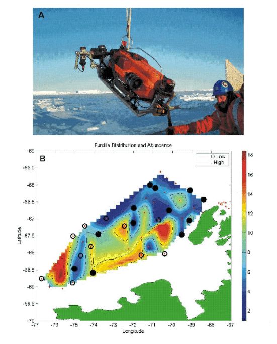 Figure 19. a) Remotely Operated Vehicle (ROV) SeaRover being deployed off the stern
of the Nathaniel B. Palmer under 10/10 ice conditions. b). Distribution and abundance of
krill furcilia (circles) plotted on top of microplankton distribution (gridded data). Open
circles indicate ROV deployments where no furcilia were observed. Closed circles
indicate where furcilia were abundant. Note that in general, where furcilia were found,
microplankton concentrations were low.
Figure 19. a) Remotely Operated Vehicle (ROV) SeaRover being deployed off the stern
of the Nathaniel B. Palmer under 10/10 ice conditions. b). Distribution and abundance of
krill furcilia (circles) plotted on top of microplankton distribution (gridded data). Open
circles indicate ROV deployments where no furcilia were observed. Closed circles
indicate where furcilia were abundant. Note that in general, where furcilia were found,
microplankton concentrations were low.Precise positioning and sizing of the target within the 0.5 m3 will be established through post-processing using a sterogrammetry algorithm (Gallager et al. 2002). The forward speed of the ROV is established with data from the ADCP and used in conjunction with the image volume to calculate volume sampled per unit time. The ADCP also provides distance to the under-ice surface, under-ice topology, and backscatter intensity. The sector scanning sonar is used to evaluate distance from the ice and for locating krill swarms. The CTD provides backup data on ROV depth and documentation of hydrography. In addition to larval distribution, swimming behavior is quantified. Stereogrammetry is used to measure swim speeds and direction to obtain a vector for each individual every 30 s-1. To correct for background motion, the instantaneous vector for all particles in the field of view are ensemble averaged and subtracted from each organism at 30 s-1 intervals. Thus the swimming speed, direction and body posture, angle of attack, etc. is quantified as a function of body size and developmental stage (Gallager et al. 2002).
We completed 26 successful deployments of SeaRover (Table 7). In general, larval krill were uncommon in the southern sector of the grid, and common in the northern sector along the under-ice surface in association with crevasses and cracks in the ice (Figure 19b). Figure 19b also shows the surface concentration of microplankton across the entire survey grid. As will be discussed in detail in the larval krill feeding experiment report below, where furcilia were abundant, microplankton were scarce. The general impression is that the furcilia concentrations are far lower than found last year on NBP0104. Only a few stations had sufficient numbers where swarms or aggregations formed. The last two deployments were part of a 24-hour process station where net hauls and CTD casts were made around the clock. The purpose of multiple ROV deployments was to determine if diel vertical migration was important to furcilia. A brief description of each deployment follows.
Table 7. ROV deployment log.
Number |
Station |
Position Lat(S)-Lon(W) |
Date |
Local Time |
Tapes |
Ctd file |
Sonar file |
ADCP file |
ROV 1 |
CS3 |
-66 33.978 -67 32.456 |
6 Aug |
0528 |
1,2,3 |
Aug62002ctd |
Aug62002sonar |
31031r |
ROV 2 |
CS4 |
-66 31.882 -67 38 188 |
7 Aug |
0849 |
4,5,6 |
Aug72002ctd |
Aug72002sonar |
31032r |
ROV 3 |
Tran 1 |
-67 13.369 -70 38.604 |
9 Aug |
1700 |
7,8,9 |
Aug92002ctd |
Aug92002sonar |
31033r |
ROV 4 |
Sta 77 |
-68 51.75 -75 7.073 |
12 Aug |
1824 |
10,11,12 |
Aug12202ctd |
Aug12202sonar |
31034r |
ROV 5 |
Sta 82 |
-68 46.724 -76 46.911 |
14 Aug |
0544 |
13,14,15 |
Aug14202ctd |
Aug14202sonar |
31035r |
ROV 6 |
Sta 72 |
-68 35.553 -74 05.097 |
15 Aug |
2210 |
16,17,18 |
Aug15202ctd |
Aug15202sonar |
31036r |
ROV 7 |
Sta 65 |
-68 05.493 -74 44.720 |
17 Aug |
0821 |
19,20,21 |
Aug17202ctd |
Aug17202sonar |
31037r |
ROV 8 |
Sta 42 |
-76 33.056 -71 36.280 |
19 Aug |
0519 |
22,23,24 |
Aug19202ctd |
Aug19202sonar |
31038r |
ROV 9 |
Sta 43 |
-67 15.705 -72 31.354 |
20 Aug |
0727 |
25,26,27 |
Aug20202ctd |
Aug20202sonar |
31039r |
ROV 10 |
Sta 44 |
-76 01.285 -73 24.595 |
21 Aug |
0334 |
28,29,30 |
Aug21202ctd |
Aug21202sonar |
31040r |
ROV 11 |
Sta 45 |
-67 10.101 -74 28.443 |
22 Aug |
0515 |
31,32,33 |
Aug22202ctd |
Aug22202sonar |
31041r |
ROV 12 |
Sta 64 |
-67 30.819 -75 06.352 |
23 Aug |
0857 |
34,35,36 |
Aug23202ctd |
Aug23202sonar |
31042r |
ROV 13 |
Sta 62 |
-67 48.776 -74 11.335 |
24 Aug |
0918 |
37,38,39 |
Aug24202ctd |
Aug24202sonar |
31043r |
ROV 14 |
Sta 49 |
-68 03.083 -71 33.400 |
25 Aug |
1719 |
40,41,42 |
Aug25202ctd |
Aug25202sonar |
31044r |
ROV 15 |
Sta 40 |
-67 56.240 -70 53.859 |
27 Aug |
2005 |
43,44,45 |
Aug27202ctd |
Aug27202sonar |
31045r |
ROV 16 |
Sta 26 |
-67 06.827 -72 00.226 |
29Aug |
0400 |
46,47,48 |
Aug29202ctd |
Aug29202sonar |
31046r |
ROV 17 |
Sta 4 |
-66 09.830 -69 04.797 |
1 Sept |
0253 |
49,50,51 |
Sept1202ctd |
Sept1202sonar |
31047r |
ROV 18 |
Sta 13 |
-65 59.739 -71 03.421 |
3 Sept |
0149 |
52,53,54 |
Sept2202ctd |
Sept2202sonar |
31048r |
ROV19 |
Sta 12 |
-66 06.163 -70 52.343 |
3 Sept |
0712 |
55,56,57 |
Sept3rov19ct |
Sept3rov19sonr |
31049r |
ROV 20 |
Sta 16 |
-66 44.746 -70 10.327 |
4 Sept |
1736 |
58,59,60 |
Sept4202ctd |
Sept4202sonar |
31050r |
ROV 21 |
Sta 23 |
-66 35.955 -72 06.535 |
5 Sept |
2332 |
61,62,63 |
Sept5202ctd |
Sept5202sonar |
31051r |
ROV 22 |
Sta 21 |
-76 02.617 -70 42.813 |
6 Sept |
2359 |
64,65,66 |
Sept6202ctd |
Sept6202sonar |
31052r |
ROV 23 |
Sta 17 |
-66 58.335 -69 29.787 |
8 Sept |
2036 |
67,68,69 |
Sept8202ctd |
Sept8202sonar |
31053r |
ROV 24 |
Sta 5 |
-66 24.316 -68 22.727 |
9 Sept |
2331 |
70,71,72 |
Sept9202ctd |
Sept9202sonar |
31054r |
ROV 25 |
RI 1 |
-65 10.382 -65 37.560 |
11 Sept |
0909 |
73,74,75 |
Sept11202ct |
Sept11202sonar |
31055r |
ROV 26 |
RI 2 |
-65 07.709 -65 30.728 |
12 Sept |
0046 |
76,77,78 |
Sept12202ct |
Sept12202sonar |
31056r |
6.3.2 Description of individual deployments
ROV 1, Station CS3. 6 August 2002, 0528 h: We deployed in Crystal Sound at 0528 hours local time at CTD Station 3 in conjunction with setting up an ice camp for obtaining cores. All systems operated correctly as the ROV traversed along three radial transects to the starboard side of the ship, each a distance of about 100 m. The ice was about 65 cm thick with a snow cover of another 50 cm. The underside was rough and jagged with protrusions extending 3 to 4 m downward interspersed with regions of relatively flat surface. Usually we find larval krill (furcilia stage 5 and 6) concentrated in the nooks and crannies along with swarms along the bottom edge of the deepest protrusions, but today not a single furcilia was observed. Only a single ctenophore about 1 cm in diameter drifted by during the deployment. These observations confirmed those of the dive team who also reported the striking lack of furcilia under the ice. The area of deployment was in the southern region of Matha Strait where a strong current typically runs into Crystal Sound. Although Crystal Sound typically has an abundance of furcilia this time of the year, the Strait may be a region of transport and not retention as found in the inner Sound.
ROV 2, Station CS 4, 7 August 2002, 0849 h: The second ROV deployment in Crystal Sound took place at 66 31.882S; 67 37.980W at CTD Station 4. At 0849 the release pin was pulled between the ROV pick up point and the aft crane used to swing the SeaRover over the starboard quarter. Three transects about 80 m each were conducted radially out from the ship into loosely packed ice and then under a large floe. Krill furcilia were observed in scattered groups near the edges of the 1 m thick floe and in the unconsolidated material, but not within the smooth, interior regions. Furcilia groups ranged in density from 10 to hundreds of individuals, but this is certainly not the greatest numbers we have seen. One ctenophore was observed about 1 m from the under surface of the ice in a particularly rough and jagged region of the transect. The ADCP showed strong, 1 kt current to the West out of Crystal Sound which may be responsible for carrying larval krill off the shelf. The deployment was cut short after 75 minutes since the R/V Gould was ready to leave and the ice team, working on the large floe to the starboard side of the ship, was back on board.
ROV 3, Transit Station 1, 9 August 2002, 1659 h: While waiting for penguins to be captured by Gould scientists and the ice team to take cores from the Palmer, we had a quick response opportunity for another ROV deployment. At 1659, while locked in ice at 67 13.369S; 70 38.604W, the SeaRover was deployed over the stern by the starboard crane. The ice was approximately 1 m thick with 50 cm snow cover that blocked the penetration of any remaining ambient light in the late afternoon hours. Four transects were made extending out approximately 100 m from the starboard quarter in a radial pattern. The under-ice topography was very rough with ridges and jagged edges jutting down to a depth of 6 m. The ROV traveled about 3 m below the ice under-surface scanning with its stereo cameras, ADCP current meter, and sonar system for larval krill (furcilia) and their predators. Furcilia aggregations appeared sporadically along the transects with organism density ranging from 10 to a few hundred individuals per group. The larvae were generally nestled up into the nooks and crannies of the jagged ice, but occasionally appeared in dense aggregations at the bottom tips of an ice projection. Such aggregations are probably caused by an interaction between water flow characteristics around the projection and swimming behavior of the individual furcilia. No furcilia were observed while the ROV traversed regions of smooth ice. Ctenophore predators were observed about 1 to 2 m below the ice under surface with tentacles extended. Body diameters were on the order of 1 to 2 cm but full quantification of abundance and size must await further data processing. A number of large amphipods swam through the light beam and attached to the ice surface, remaining attached for 10s of seconds. The entire deployment required 70 minutes from start to finish with 58 minutes of actual surveying time. A photograph was taken from the helodeck to qualify the ice conditions.
ROV 4, Station 77, 12 August 2002, 1824 h: This deployment was at Station 77 with open leads, grease ice, and thin ice floes. At 1824, the ship positioned itself in a lead with thick ice on either side. The ice team went over the side followed by the ROV. The Simrad and ADCP acoustic systems showed strong scattering at 300, 150 and 100 m but not near the surface. The under-ice surface was smooth in the region of a floe, and jagged under ridges. Some second year ice was observed with dark layers intermixed with light ice layers, particularly on edges 50 cm thick or greater. Some furcilia were in the water column. The occasional larva swam by with no aggregations of organisms in the many pockets created by the ice ridges. Fish larvae were abundant, swimming within the deeper pockets and ice shelves. A few ctenophores, with tentacles extended, floated by the cameras view. The habitat afforded by the many nooks and crannies screamed krill country, but large aggregations of krill were not to be found. The ROV was taken out of the water at 1951.
ROV 5, Station 82, 14 August 2002, 0509 h: This station was characterized by thick ice, high ridges, and small compacted floes. The wind was hovering around 35-40 kts in near whiteout conditions as the ROV was deployed off the starboard quarter at 0509. Deployment of the ice team was delayed due to the wind conditions. The ROV had been sitting on deck waiting for the crane operator for half an hour and had reached the ambient temperature of –20 C. When the ROV hit the water a spray of newly formed ice exploded off the metal parts into a convective plume billowing up from the vehicle. A thick layer of ice immediately formed on the stereo camera windows causing a blackout on the control monitors. Since we had not as yet pulled the release pin, we were able to bring the ROV up to the level of the gunwale and spray the windows with alcohol and a soap solution. The alcohol lowered the melting temperature while the surfactant in the soap prevented new crystals from forming on the glass surfaces. The ROV was put back in the water and released within a few minutes. A Crabeater seal played in the vicinity of the ROV during the entire deployment, frolicking in the intense light of the strobe. Unfortunately, this was the only organism observed during this deployment. Not a single furcilia, ctenophore, fish larva, or isopod was seen.
ROV 6, Station 72, 15 August 2002: Station 72 was characterized by thick ice, high ridges, and small floes. A few furcilia seen under ridges. No major swarms were observed, but on order 2 to 100 individuals per cubic meter. A few ctenophores and fish larvae were also seen.
ROV 7, Station 65, 17 August 2002, 0809 h: Station 65 was characterized by 10/10 ice cover, moderately high ridges on the order of 1 to 2 m, and small, compacted floes about 10 to 50 m across. The wind was low and the ambient temperature was only -8 oC as the ROV was deployed off the starboard quarter at 0809. The ice team was deployed immediately before launching the ROV. The ROV descended to 20 m and began its transects at a heading of 45o off the starboard side towards the bow of the ship. The ships gyro compass read 26o. Upon reaching the end of the 150 m tether, the ROV turned to the right 90o and began sweeping the undersurface of the ice while following within 3 m of the ice interface. Six transects of about 70 m each were made parallel to the ships axis in undisturbed ice. The smooth but pock marked under-ice surface of floes gave way to deeply protruding ridges extending 4 m in depth. Although this was not the most extensive ridge field encountered on this cruise, the 1 m thick jagged edges standing vertically were impressive. Some brown ice layered with clear ice was encountered. The first transect presented little in the way of plankton, only a few ctenophores. The second through fourth transects found numerous larval fish hovering about 0.5 m below the ice under-surface and not up in the nooks and crannies provided by the rafted ice. Although these larvae did not appear to be aggregated, they did occur in groups of about 3 to 10 at a time. A relatively strong current of about 1 kt made it difficult to stay with the larvae for more than a few seconds, but considerable stereo video footage was obtained for extraction of swimming vectors. No larval krill were observed on this deployment. Towards the end of the deployment, 1st Mate Mike Watson on the bridge asked to have a look at the opening to the moon pool and the covers to the new Simrad acoustic system. As ship's engineers John Pierce and Dave Munroe watched the ROV camera monitors and provided directions in what can be a complicated environment, the ROV traveled along the hull on the starboard side of the ship. Numerous devices used for cathodic protection were located along the hull. Some areas of the hull apparently not painted during the recent dry dock due to positions of under hull supports were also noted. The moon pool was jammed with ice chunks about 0.5 to 1 m in diameter that protruded below the hull's surface by about 0.75 m. The horizontal cover to the Simrad was located just forward of amidships. The cover was bright yellow and covered with flat ice chunks about 20 cm thick by 0.5 m wide. Attempts were made to push away the ice to get a better look at the cover but the buoyancy of the ice made it surprisingly difficult to move the chunks away from the cover. It was almost as if the ice was cemented in place. As the ROV was repositioned to the forward side of the cover, it began to feel the current generated by the ships forward thruster that was being used to keep the ship up against the ice. It was decided to dive quickly to get any slack tether out of harms way. The dive ended by motoring back to the stern followed by an uneventful retrieval by the deck crew using the starboard knuckle crane.
ROV 8, Station 42, 19 August 2002, 0519 h: ROV deployment 8 was interesting in a number of respects. The Gould was positioned in the area waiting to hear a report on furcilia abundance before deciding to remain at their location and execute a dive, or to move on to another station. The Palmer left the Gould in a large open water lead about 0400 local time to find a suitable ice floe for both ice work and an ROV deployment. By 0500 we were pulling into a mass of thin new ice followed by thicker 2nd year ice formed into small but thick flat surfaces. An extensive ridge line about 2 m in height separated each floe, which appeared clearly on the ship’s high resolution radar. After positioning next to a 2nd year floe about 50 m across, the ice team was deployed followed immediately by the ROV at 0519. The ROV made its way through an extensive ridge field while traveling on a bearing directly under where the ice team was working. After crossing the ridge at a depth of 11 m, the ROV ascended to 4 m to find a near mirror smooth surface dimpled with 10 cm diameter depressions. From distance calculations this was the area where the ice team was working. We had talked about putting a pole through the ice after the first hole was drilled so the ROV could get a good look at the defined area, but this was not done in this deployment. In any case, the color video footage may be useful in characterizing the under surface at a later time. Furcilia were present in numbers ranging from 2 to 20 individuals per image window translating into a maximum of 40 per cubic meter. Small groups of furcilia appeared deep at the tips of the overhangs and ridges around 10 m deep. Small numbers of individuals were scattered throughout the upper water column (12 m deep) and up to the ice under surface. By far this was the greatest concentration of furcilia we have observed on this cruise including all the southern stations. However, the observed concentration was considerably lower than the extremely dense aggregations observed on NBP0104 one year ago where numbers exceeded 17,000 individuals per cubic meter on several occasions. Following the deployment, these observations were reported by radio to researchers on the Gould who decided to go ahead with the dive and attempt to collect furcilia for growth experiments. As a side note, the ridge field in this area was extremely dense and complicated under water making navigation difficult. More than once the tether caught on ledges and overhangs requiring some quick maneuvering to keep from entanglement. We removed a few of the floats from the tether making is a little less buoyant with the hopes of keeping it out of harms way.
ROV 9, Station 43, 20 August 2002, 0727 h: This region was characterized by 1 m thick, small, refrozen ice floes about 10 to 20 m in diameter with an extensive ridge field on the order of 1 to 2 m high. These characteristics proved difficult for the ROV to operate in because of the dangers of tether entanglement on the extensive 3 dimensional structures below. The bridge also had a difficult time finding stable ice on which to deploy the ice team since cracks appeared quickly after the ship began to penetrate the area. After three attempts, a solid floe was located and we were off. First the ice team landed on the ice and then the ROV went into the water at 0727. Before the deployment, the bulb for the high intensity strobe on the 3D camera needed to be replaced. This required about 20 minutes of extra time on the deck allowing the temperature of the vehicle and cameras to reach air temperature of –27oC. Upon entering the water, ice crystals formed on the metal parts and roared to the surface in a violent plume. The glass camera windows iced over with an opaque layer which looked like someone had painted the windows black. The ROV was removed form the water, the camera windows sprayed with ethanol to dissolve the ice, and replaced in the water. The first hour of the dive was spectacular as the ROV ascended into cavernous under-ice domed structures constructed of rafting floes. As we moved through our transects there were scattered furcilia up in the shallowest regions and small groups of 5 to 10 individuals located at 8 to 10 m depth immediately below the deepest ridges. Small numbers of ctenophores drifted by followed by the occasional fish larva. The under-ice surface of the floe being worked on by Frank Stewart and the ice team was smooth with the exception of pock marks 10 cm or so in diameter. A small number of single furcilia floated by with no signs of aggregations. The ridge line was clearly visible on the ROV-mounted sonar system allowing good measurements of floe and ridged surfaces. The ROV then moved into some unconsolidated brash and bergy bits on order 2 to 10 m in diameter. Furcilia were present in low numbers (approximately 2 to 10 individuals per cubic meter). The brash was moving around a bit with the 1 kt current. Soon the ROV discovered that it could neither move up, down or laterally within this minefield of ice. The tether could be seen to have lodged into several crevasses in front of the vehicle and additionally behind the vehicle, in its blind spot, keeping it on a short leash. We worked for several hours maneuvering in and around the ice blocks and ridges trying to untangle the trapped tether. A clump weight was dropped down the tether from the ship in an attempt to lower the point of insertion and free at least one end. Several times during this ordeal we gained some tether giving us the false impression that we had been freed. However, as one region of the tether was freed, additional entrapment points became evident. We were faced with three options: Send in the divers who might be able to free the tether, but possibly at the same time jeopardize their own safety in this difficult environment. Another thought, provided by Chief Scientist Peter Wiebe, was to very gently turn the ship screws and get the water moving behind the ship just enough to cause the brash to move and possibly free the tether without damaging the vehicle. The last possibility was to cut the tether and send the ROV on its own. We decided to go for the second idea. First Mate Mike Watson deftly engaged the screws and put on 5 degrees of pitch at low rpm. After a minute, we could see from the cameras on the ROV that the brash was moving. The deck crew continued to tug on the tether and the ROV dove hard. Suddenly, we could see daylight off in the distance and we knew we were free. The ROV was retrieved, but sustained some damage to a thruster due to being jammed with ice. A spare thruster was swapped for the damaged one and we were ready to go by the time we arrived at the next station.
ROV 10, Station 44, 21 August 2002, 0519 h: ROV deployment 10 was cut short at Station 44 because the current overload indicator lights on two thruster motors, starboard and lateral, showed that a water leak had probably occurred and needed attention before continuing. The ROV was retrieved 20 minutes after entering the water, but not before making some observations of furcilia abundance close to the ship. Approximately 1 to 2 individuals were present most of the time the vehicle was close enough to the surface to have the 3D cameras in focus. No observations were made at depth since we were making preparations for immediate retrieval. Following retrieval, the two offending thruster motors were removed, cleaned and refilled with a special oil to keep water from entering the shaft housing.
ROV 11, Station 45, 21 August 2002, 0603 h: Offshore Station 45 was characterized by small 2nd year floes broken and refrozen with many ridges about 1 to 1.5 meters in height. Open leads approximately 50 m wide were observed 200 m to our starboard and port sides. The ROV was deployed at 0603. After a brief period of thruster and buoyancy testing the hook was pulled and off we went to the south, 90o to the axis of the ship. The ROV had recently undergone some rebuilding due to thruster malfunction so this was predominantly a quick system checkout dive, but the opportunity existed to collect data while testing. Two 40 m transects were conducted. No furcilia were observed either at depth or up into the crevasses of intertwined ridges and rafted blocks of ice. Most ice appeared rounded and smooth rather than sharp and jagged indicating older ice that has undergone some melting, and refreezing. Two or three ctenophores floated by at a depth of 12 m, but no larval fish or furcilia aggregation were observed at this offshore site. The strobe bulb on the 3D camera system blew out at the end of the second transect bringing this deployment to an end. The strobe was re-lamped and made ready for the next deployment at Station 47.
ROV 12, Station 64, 23 August 2002, 0857 h: Ice conditions at offshore Station 64 (-67 30.819S; –75 06.352W) were similar in some respects to those of Station 45. The ice was characterized by small (10 to 20 m diameter) second year, or older, floes composed of broken and refrozen brash. Between floes an extensive network of snow covered ridges extended to a height of about 1 to 1.5 meters. Open leads approximately 50 to 100 m wide were present along with numerous small, rounded and weathered icebergs with diameters on order 100 m. The ROV was deployed at 0857. Following checkout of all systems, the release pin was pulled and the ROV headed toward the small ice flow on which the ice team was currently working. On the way over to the floe, the ROV dove under two ridges which extended to a depth of 12 m. Ascending to a depth of 3 m on the other side, we found the underside of the floe was not the typical smooth surface associated with floes previously observed, but a conglomeration of smaller flat ice chunks re-frozen into a solid mass. Dark coloration penetrated deeply into the ice. Another distinct feature of this area was that the ridges, which appeared as solid masses from above, were actually very loosely organized with large gaps between the rafting chunks. These gaps were covered in snow from above but allowed a substantial amount of light to penetrate to depth. While the ROV hovered at a depth of 40 m with its headlights turned off, the extensive network of ridges could be seen highlighted by sunlight penetrating through the snow, making it appear like a patchwork quilt of various sizes and shapes. The edges of the brash and rafting ice were worn smooth and were not sharp as typically seen when first year ice is broken. Unfortunately, as enticing as this may have seemed as potential krill habitat, not a single furcilia larva, ctenophore or fish larva was noted along three series of transects totaling more than 350 m covered by the ROV.
ROV 13, Station 62, 24 August 2002, 0918 h: Today’s deployment was near Station 62 (–67 48.776S; –74 11.335W) directly over the shelf break. The 10/10 ice cover was characterized by small (5 to 20 m diameter) second year floes composed of broken and refrozen brash. Between floes, an extensive network of snow covered ridges extended to a height of about 1 meter. A few small open leads were present along with numerous small icebergs with diameters on order 100 m. The ROV was not scheduled for this station, but we decided that the results of a short deployment would be useful to both the divers and trawlers in deciding what should be attempted at this station. The ship drove into an area of re-frozen floes and became stationary at a heading of 149o. The ROV was deployed at 0918 immediately after the ice team began their work on a small floe on the starboard side of the ship. Following checkout of all systems, the release pin was pulled and the ROV headed towards the small ice flow on which the ice team was currently working. There were three seals frolicking in the pool behind the ship and took quite an interest in the ROV. Video footage was acquired on both the large area color pan and tilt camera and the 3D stereo cameras of the seals swimming by and checking out this odd looking co-habitant of their underwater world. The ROV dove to 30 m quickly and traveled under a series of ridge lines, then came to the under surface at 8 m and began a transect on a magnetic bearing of 220o. In all, four transects were conducted each approximately 40 m long and parallel to the ship’s axis. The seals did not follow the ROV under the ice ledge. The under-ice surface was characterized by thick, flat plates rafted on top of one another and refrozen into a solid mass. There were many complicated channels and domed chambers that the ROV explored as fully as possible. Once again, however, not a single larval krill or other plankter was observed. The next station is 49 about 20 nm from the mouth of Marguerite Bay.
ROV 14, Station 49, 25 August 2002, 1719 h: Today’s deployment was near Station 49. The ice was characterized by broken and refrozen floes extensively rafted into many layers. The ROV went into the water for a short deployment at 1719 local time and was retrieved at 1812. A problem with the strobe light delayed the deployment 40 minutes as we found some electronic parts and a new bulb to replace one that apparently had blown out. We later discovered that the problem was not a blown bulb but a temperature sensitive part in the power supply and control housing for the 3D VPR cameras and strobe. A few activated hand warmers tossed into the housing provided the extra heat necessary to keep the power supplies above –20 oC for this deployment. We developed a ceramic heater to be installed in the electronics housing for future deployments. No furcilia were observed either on the relatively flat regions of the small floes or in the rough, complicated environment of the rafted and buckled ridge lines. A few small ctenophores were scattered throughout the dive.
ROV 15, Station 40, 27 August 2002, 2005 h: After a day of intensive backing and ramming the ship became free from the heavy grip of high pressure ice at Station 40. A few miles away from Station 40, on our way to Station 28, we stopped for an ice team and ROV deployment ( –67 56.240S; –70 53.859W). The air temperature was relatively warm at –6.2 oC so the newly installed ceramic heater in the power supply electronics housing of the 3D camera system was not necessarily tested under extreme conditions. However, the strobe functioned normally so we were hoping the heater had solved our immediate temperature sensitive problem. The ice was characterized by large, flat floes of first year ice about 70 cm thick. A ridge line appeared about 500 m on the starboard side of the ship but was too distant for the ROV to reach. The under-ice surface was quite smooth and dimpled, without rafting of any kind. A few cracks opened by ship activity showed the ice floe to be layered, but not extensively with colored material. One corer used by the ice team was observed from below by the ROV. This observation was short-lived as the corer was lost as it fell through the ice and down to the bottom. Another bore hole was found after the ice team inserted a flag pole for the ROV to identify. One ctenophore and one seal were observed, but no larval krill.
ROV 16, Station 26, 29 August 2002, 0425 h: Early on the morning of the 29th, we deployed the ROV near Station 26 (–67 06.827S; –72 00.226W) where the bottom depth was 323 m. The area was 10/10 ice-covered with small re-frozen floes and extensive ridge fields about 1 m in height. Ice thickness was about 1.2 m with 30 cm snow cover. The ROV was deployed at 0425 local time immediately after the ice team landed on a small floe on the starboard side of the ship. Once in the water, the ROV instrumentation and sensor systems were checked out and a transect was started at a bearing of 90 deg with the ship’s bow positioned at 47 deg. A ridge 12 m deep was navigated immediately upon leaving the aft end of the ship. Within an additional 50 m, the bottom of the flow where the ice team was working appeared on our screens. The undersurface of the floe was very heterogeneous, rough and jagged, appearing like re-frozen brash and chunks, rather than the smooth surface characterizing floes of first year ice. Furcilia stages of krill larvae were scattered throughout the area at concentrations between 0.5 and 5 per cubic m. One to three furcilia were observed every few seconds on the stereo VPR camera system. There were no large aggregations or patches of furcilia. Most larvae were motionless angled sharply forward in a head down position, but a few were swimming slowly at an attack angle of about –30 deg. Many ctenophores were also observed on order 1 per cubic m. Most furcilia and ctenophores were relatively deep at the tips of the ridges rather than up against the undersurface of the floes. We conducted a Reeve net haul to capture some furcilia for feeding experiments.
ROV 17, Station 4, 01 September 2002, 0253 h: Early this morning at 0253 local time, we deployed the ROV near Station 4 (–66 09.830S; –69 04.797W) where the bottom depth was 450 m. Ice cover was 10/10 but characterized by small floes (<10 m) bordered by open leads and brash. Significant ocean swell was observed rolling through the ice apparently keeping the ice from re-freezing. The swell kept the ship in constant motion making positioning against a floe difficult. The ice was deemed too thin to put the ice team on a floe so the ROV went in without its company. The Reeve net was used immediately prior to the ROV deployment and had caught large numbers of krill furcilia so we knew we had a chance of observing significant numbers during this survey. The first transect extended at a bearing of 300 degrees and range of 40 m directly abeam on the starboard quarter. Furcilia were scattered throughout the water column all the way from just under the ice to 10 m depth. There were no significant ice ridges so the furcilia were not being concentrated in any particular location. About 3 to 50 furcilia were in view most of the time resulting in concentrations of 6 to 100 per cubic meter. Most individuals were small (<1 cm), probably Stage 5 or 6 furcilia, but an occasional juvenile 2 cm in length swam through the field of view. Towards the outer region of the transect grid, furthest away from the ship, the ROV characterized at least five relatively dense swarms consisting of more than 500 individuals and generally hanging immediately below or at the edge of a small open lead. The swarms were about 10 to 15 cm in diameter and loosely compacted (nearest neighbor distances were at least one body length). The local concentration was about the same as observed last year on NBP0104 for the smallest swarms. Furcilia within the swarms appeared to be alternating between swimming up and then down as if they were following water currents associated with the tilting of the floes in sea swell. In contrast, those larvae separated from groups and freely drifting under more open areas of the under surface were generally positioned head down at an angle of about –30 degrees, and not swimming. Both large and small ctenophores were plentiful, drifting about 50 to 100 cm below the under-ice surface. Attempts were made to maintain the 3D cameras on the ctenophores and observe behavior of ctenophores feeding on krill larvae. Three video segments for more than two minutes each were made while following single ctenophores. The last segment contained a large ctenophore about 8 cm in body length with tentacles extended over 1 m with a furcilia caught in one tentacle. The ctenophore’s body was undergoing end for end cartwheels and axial rotations in an attempt to entangle its prey and bring it up to its mouth. Unfortunately, the quarry was lost before ingestion could be observed. The data from this deployment will be very useful for determining swimming speeds and orientation relative to swarm size.
ROV 18, Station 13 , 03 September 2002, 0150 h: This was the first of back-to-back ROV deployments at the offshore Station 13 (ROV18) and the shelf break Station 12 (ROV19). At Station 13 (-65 59.793S; -71 03.421W), the ice was characterized by small floes drifting with the wind and separated by narrow open leads and brash. Ocean swell caused the floes to remain separated rather than re-freezing into a consolidated mass. The ROV was deployed at 0150 local time. There were small numbers of furcilia drifting throughout the area, but they tended to be concentrated up in the open leads and brash and along edges of the broken floes. Concentrations were low, approximately 1 to 10 per cubic meter. Four or five ctenophores and some amphipods were also present in the area.
ROV 19, Station 12, 03 September 2002, 0712 h: The second deployment of the morning was at Station 12 (-66 06.163S; -70 52.343W). The ROV was deployed at 0712 local time just as first light appeared on the horizon. Ice conditions were very similar to those of Station 13; small floes held apart by ocean swell. There were many more furcilia at this station, but unlike the previous location, the larvae were located at depth beneath the deepest ice projections rather than in the open leads and brash. Given the early morning conditions, it is possible that the larvae migrated to deeper regions of the ice pack (10 m). However, we have not observed vertical migration in krill larvae and we suspect that there is little if any effect of time of day on their distribution. One striking feature of this station was the varied size structure of the larval populations. Furcilia Stages 4 through 6 and even some juveniles were present synoptically. A Reeve net tow made immediately before this deployment, however, provided evidence for juveniles of Thysanoessa sp. rather than Euphausia superba, so the species of the larger krill observed by the ROV remains in question.
ROV 20, Station 16, 04 September 2002, 1730 h: ROV 20 was a late afternoon (1730) deployment at Station 16 (-66 44.746S; -70 10.327W). Ice conditions were 9/10 ice cover with 10 to 50 m diameter floes and compressed ridge lines. The ice team was working on a large floe next to the ship as the ROV was deployed and began a transect out to a ridge line about 100 m to starboard. As the ROV traversed the undersurface of the floe, we observed a smooth undersurface and no furcilia larvae. Just as the edge of the floe and junction with the ridge line was approached, swarms of furcilia appeared in view. The larvae were small, possibly Stage 4 or 5 and formed dense aggregations in direct contact with the ice. The ice itself was different in that the light from the ROV was absorbed and not reflected back to the cameras as observed under most conditions. Internal reflectance is common in ice in the process of melting and forming brine channels. The ROV continued down under the ridge and began a transect to the south along the axis of the ridge. Throughout this transect, no furcilia were observed. It was as if they had disappeared. The ROV turned again 90 deg to starboard on a bearing taking it back across the open floe surface. As the junction between the ridge line and flow was approached, again there were masses or furcilia forming just below the ice surface. The ROV continued back to the stern of the ship and began a fourth transect at a bearing heading for where the ice team was working and had established a transect line of bore holes. The first bore hole was encountered with help from the bridge calling out positions of the ROV strobe light seen through the 1 m thick ice. A pole was inserted from above as the ROV documented depth penetration and characteristics of the ice surrounding the bore hole. The bridge again called out a bearing to the next bore hole on the transect and the ROV began the search. This was repeated five times until the last bore hole was located about 90 m from the ship at the floe/ridge junction. Chris Fristen had an auger extending through the last hole, which was drilled through multiple layers of rafted ice. Krill furcilia were abundant in the area around the hole as the auger was repeatedly removed and replaced in an attempt to suck some furcilia through the hole. Ctenophores and a few larval fish were also present where furcilia were abundant. These observations support the idea of a combination of biophysical processes which control the under-ice distribution of larvae. It is likely that as the water flow across the flat surface is disturbed by the ridge line, small eddies and counter currents develop extending 1 meter or more from the ice. The swimming behavior of the larvae interacts with the physical flows to produce aggregations at certain positions. Furcilia larvae are rheotactic, meaning that they orient into and swim against a water current just as fish do in a stream. As the furcilia swim against the local water flow generated by rapid changes in ice topology, their retention time in that particular part of the flow increases causing a localized increase in larval concentration. This increase in local concentration is what we refer to as an aggregation. The larvae become concentrated in the same area of the flow simply because they have similar swimming behaviors. Whether there are other biological cues involved in initiating or maintaining such aggregations are unknown. Aggregations of larvae are in contrast to the large masses of adult krill referred to as swarms. Biophysical processes similar to those described for the larvae may initiate a swarm, but intensification and persistence of the swarm is most likely augmented by both chemical and mechanical signals generated as a result of swimming and for reproduction.
ROV 21, Station 23, 05 September 2002, 2332 h: ROV deployment 21 was performed at Station 23 (-66 35.955S; -72 06.535W) in the presence of small re-frozen floes amongst pancake ice and freshly formed brash. Four 60 m transects were performed out from the starboard side of the ship. In general, very small numbers of krill furcilia were found at this offshore station. The big surprise was the observation of juvenile and adult krill in fairly large numbers ranging from directly under the ice to a depth of 60 m. This was the first time older individuals have been seen under the ice in any great number. About 20 to 30 individuals were present in the field of view of the main ROV camera at any one time, translating into a concentration of greater than 100 per cubic meter.
ROV 22 , Station 21, 06 September 2002, 2345 h: ROV deployment 22 was performed at Station 21 (-67 02.617S; -70 42.813W). From the surface, the ice was 10/10 coverage with medium sized (10 to 100 m) first and second year floes 50 to 75 cm thick interspersed with re-frozen leads and compressed ridges 1 to 1.5 m in height. The ice team was deployed at 2345 local time followed immediately by the ROV. As the ice team drilled a transect of bore holes from the ship out to a ridge line 100 m off the starboard side, the ROV began a series of transects out under the relatively smooth section of the floe and across the ridge line. Once at the ridge line, the ROV turned aft and followed the ridge for 90 m, then turned towards the ship and came up adjacent to the starboard stern. This loop was repeated at two distances from the ship, approximately 90 m and 40 m. The ice team inserted a 4 m long bamboo pole through the most distal bore hole as a marker for the ROV which was located on the second transect loop. In contrast to Station 16 just 40 nm to the northeast, very few furcilia were observed at Station 21. A few scattered individuals drifted across the relatively smooth surfaces of the ice floes, but no aggregations or swarms were located along the ridge line. A few ctenophores drifted by, but not in remarkable numbers. Until we continue towards the coastline of Adelade Island, it will be unknown if this condition is an artifact or an indication that the furcilia are indeed found more offshore than inshore within the northern sector of our survey grid.
ROV 23, Station 17, 08 September 2002, 2036 h: ROV deployment 23 was performed at Station 17 (-66 58.335; -69 29.787). From the surface, the ice was 60/40 coverage with medium sized (10 to 100 m), broken first year floes 50 cm thick rafted into deep piles interspersed with open water leads. After checking all systems the ROV was deployed at 2036 local time only to find that the port thruster was producing a current overload. When this happens it means that water has entered the motor most likely through the lip seal of the main shaft. One of two things can occur: the thruster will continue to function but eventually burn itself out because of the excess current draw, or the thruster motor controller board in the main body of the ROV will overload and burn out a power transistor. The procedure when this happens is to shut off the controller for the bad thruster inside the topside power pack, which we did. This left the ROV unable to follow a straight course and able to turn only in the direction of port. Realizing there would not be time to retrieve the ROV and repair the thruster and get back into the water at this station, we positioned the ROV facing aft and began a transect in a slow arc out away from the ship and then back in towards the starboard side about the position of the A frame. This worked well so we repeated the operation with a longer tether lead and followed another arc shaped transect. The ice was rafted deeply so it was difficult to remain at one depth. However, even with these shortcomings, we were able to complete two 100 m long transects. Unfortunately, the furcilia abundance was low with scattered animals below even the more rugged surfaces. The concentration was roughly 1 to 2 per cubic meter. A few ctenophores were noted but they were not in high abundance. The ROV was retrieved and the port thruster repaired by draining the oil-filled housing, rinsing with fresh oil, and refilling. This operation required about 45 minutes before we were back in action and ready for the next station.
ROV 24, Station 5, 09 September 2002, 2332 h: ROV deployment 24 was performed at Station 5 (-66 24.316; -68 22.772), the last station on the northern sector of the grid. Surface ice conditions were 40/60 coverage with flooded floes and open leads. The ROV was deployed at 2332 local time in a 25 kt northeast wind, –19o wind chill, and blowing snow. The deck crew was prepared with goggles and face covers to guard against the harsh conditions. All the tether was paid out as the ROV swam directly away form the starboard quarter and dove to 8 m where a good view of the under-ice surface could be attained. The under-ice surface was surprisingly rough given the smooth conditions observed from the surface. During the first transect, a few small swarms of 50 to 100 furcilia were noted embedded in the upper ice crevasses. The ROV turned 90 degrees towards the bow of the ship and proceeded on a bearing of 30 degrees. A strong current was taking the ROV to the north and eventually under the ships hull. This would not have been a problem except that the tether had, in the meantime, wrapped around the starboard rudder and through the opening between the two main screws. The ROV tether had become lodged between the ships hull and a large block of ice up under the hull just forward of amidships. The ensuing oneand a half hours were a bit tense as we jockeyed around to get a better look at the snag. Unfortunately, the scope between the snag and the ROV was short enough to prevent turning a full 180 degrees. First Mate Mike Watson, Ice Pilot Vladimir Repin, Second Mate Paul Jarkiewkz, and Third Mate Rachelle Pagtalunan, all were observing the conditions and suggesting potential moves. In a final attempt to dislodge the ROV, Captain Joe began gently swinging the forward thruster back and forth towards starboard side and aft. Within a few seconds, we could see water moving past the ROV. The ROV dove hard and suddenly we could feel some freedom in the tether. With the ROV at a safe depth of 40 m, the deck crew began pulling the tether free from the rudder. Soon, and with a sigh of relief, the deck crew reported the ROV lights in sight and retrieval operations commenced.
ROV 25, Station RI 1, 11 September 2002, 0909 h: ROV deployment 25 was performed at the 24 h anchor station just south of Renaud Island (-65 10.382; -65 37.560) during daylight hours. The purpose of this last set of deployments was to determine if furcilia undergo diel vertical migration. Some forms of plankton swim up into the water column at night, and down to depth during daylight hours. There are many potential reasons for this behavior, but the most likely one appears to be avoidance of visual predators during the day. Adult and juvenile krill have been observed to migrate hundreds of meters a day, but vertical migration in their furcilia stage larvae has not been observed. The Renaud Island deployments began at 0909 local time in full sunlight. The surface ice conditions were 90/10 flooded floes with 30 to 50 cm snow cover. The ice team proceeded cautiously on what could be dangerous conditions. The 1-m MOCNESS had just collected large quantities of juvenile krill in the upper 25 m and seals and penguins were sighted in the area. The ROV immediately came across large swarms of furcilia rafted up into crevasses between floes. After completing the first transect arc out to the starboard side and then aft, we came across one swarm that was in direct association with the ice surface. A small pocket about 30 cm across appeared to contain thousands of furcilia. Larvae were swarming in the water and crawling on the ice surface like ants on a dirt mound. The ROV kept the 3D VPR cameras fixed on this swarm for more than 12 minutes allowing concentration estimates and swimming behavior observations to be conducted. Three more transect lines were completed and the ROV was retrieved after one hour 30 minutes of observations. By far this station had the greatest number of furcilia, and they were present in bright sunlight. Estimated concentrations range from 5,000 to 100,000 larvae per cubic meter in swarms and 200 to 1000 per cubic meter on average. At the end of the deployment, the ROV dove to a depth of 50 m and turned upwards to view the tapestry of patterns produced by sunlight projecting through the snow covered ridges and open leads.
ROV 26, Station RI 2, 12 September 2002, 0046 h: ROV deployment 26 was performed at the 24 h anchor station just south of Renaud Island (-65 07.709 -65 30.728) close to where ROV 25 took place but during night time hours. Surface ice conditions were the same as in ROV 25 with loosely packed floes over-flooded and snow-covered. The ROV was deployed at 0046 local time in a flurry of adult krill swarming at the surface. This phenomenon had not been observed before on this cruise so it attracted a number of people to the sides of the vessel. The ROV observed many adults, juveniles, and stage 6 furcilia, but the furcilia were not swarming as seen earlier in the day. On average about 100 to 1000 furcilia per cubic meter were observed. As a side note, divers observed very dense furcilia concentrations during the daylight hours. The conclusions based on this and all our observations of day versus night time deployments is that there does not appear to be any diel vertical migration in response to time of day or daylight in young furcilia stages. In fact, more intense swarming behavior was observed during daytime deployments than at night. One reason for this may be that larvae are attracted to light because sunlight is needed for algal growth and ice algae and microplankton are their major prey. Predator avoidance does not seem to play a major role in their behavior. The under-ice surface may provide sufficient refugia from predation and serve as a critical nursery with an abundance of food where sunlight can penetrate as a source of energy for photosynthesis. Even if the ice algae at this time of the year are not actively photosynthesizing, they could be releasing organic compounds that act as an attractant to the hungry furcilia.
6.4 Microplankton Distribution, Abundance, and Swimming Behavior
(Philip Alatalo, Gustavo Thompson, and Scott Gallager)
The objectives of our microplankton studies are: 1). To determine the vertical and horizontal distribution of autotrophic and heterotrophic microplankton, including pelagic ciliates, heterotrophic dinoflagellates, and silicaflagellates along the western Antarctic Peninsula during austral autumn and winter; 2) To provide an additional perspective on the microplankton prey field utilized by larval and adult krill, by quantifying abundance and motion characteristics, (i.e. swimming behavior) in relation to particle size distribution; 3) To relate microplankton distributions to vertical gradients in density, salt, mixing intensity, and light distribution, and horizontal gradients in water mass distribution and surface currents.
To quantify microplankton along the CTD station grid extending about 20 nm both north and south of Marguerite Bay and 20 nm offshore, we collected water using the standard 10-l Niskin bottle on the CTD rossette. CTD bottle depths for microplankton sampling were chosen keeping the following vertical regions of the water column in mind: the upper mixed layer, a fresher water lens (if present usually <20 m), the halocline at the base of the mixed layer, chlorophyll maxima and minima, and a near-bottom deep sample. Four samples were taken at each CTD station unless specific regions or strata seemed interesting based on data from the CTD, BIOMAPER-II, Simrad, or VPR. Samples were removed from the center of the Niskin bottles by gently siphoning through wide bore tubing . We have shown that this procedure minimizes damage during sample transfer particularly to large protists and aggregates (marine snow). Each depth sample was processed by preserving 200 ml in 2% Acid Lugol’s fixative and by observing swimming behavior on live, unconcentrated samples in a specially developed optical recording device. For the purpose of distinguishing between heterotrophs and autotrophs, 200 to 1000-ml samples from some stations were processed by filtration on to 0.45 um black polycarbonate filters and stained with DAPI, FITC or acridine orange. Slides were held at 0oC in the dark for a few hours until observed under fluorescence microscopy using a DAPI filter set on a Zeiss Axiophot upright microscope with 20x and 40x objectives. Digital images were saved for further counting and processing. Using DAPI stain, large heterotrophic protists appeared blue with white nuclei, while diatoms, autotrophic dinoflagellates, autotrophic, mixotrophic and other pigment-containing cells appeared also to contain a low level of orange or red fluorescence.
Automated particle tracking of microplankton from video recordings in the optical system required capturing a 30-s video sequence at 30 frames per second into an AVI file, followed by importing the AVI into a Matlab program one frame at a time. Each frame was binarized against a threshold and each “in-focus” particle’s centroid, maximum and minimum axes were recorded in a matrix. The next frame was imported and a second matrix of pixel locations was produced. A simple nearest-neighbor algorithm was then used to determine if there were particles within a certain displacement window between matrix one and matrix two. If the centroids were within the window, a particle path was created. After all paths had been created the ensemble mean velocity vector for all particles in each frame was subtracted from the instantaneous velocity vector of each particle in the field. This process removed any common mode movement associated with ship roll. A data table was created for each particle in the field for calibrated diameter, displacement, speed, motion vector, net to gross displacement (NGDR), and energy dissipation (calculated by the Lagrangian integral length scale technique). These statistics were used as characteristics in a discriminant analysis to determine associations between the swimming behavior of microplankton. The result was a description of the prey field from the perspective of the energy and frequency of motion and size distribution.
Observations from the video recording system and selected microscope slides showed a dramatic change from the early winter NBP0202 cruise. Virtually all large diatoms, dinoflagellates, and protozoans were absent from the waters of the survey grid, Crystal Sound, Matha Strait, and off Renaud Island. Very small particles with limited motility predominated at most sampled depths, especially at the top and bottom boundaries of the water column. Small flagellates exhibited most of the recorded motility, although solitary ciliates were observed occasionally. Mesodinium sp. was observed in early September, primarily in surface water at off-shore/slope stations (Sta. 1,11,12,14) in the northern section of the survey grid and at Station 9 near Adelaide Island.
During this winter time cruise, microscopic examination showed a few small diatoms (Rhizosolenia sp., Fragilariopsis sp., Chaetoceras sp.), particularly at depth and a remarkable amount of fluorescent debris, often fibrous, in the surface waters. Short diatom chains were also observed in samples collected above the thermocline or at offshore stations. Water directly associated with ice (collected by divers or at ice-stations) was typically very different: high concentrations of very small particles, including flagellates and ciliates, with low motility, but much greater than that found in CTD samples. An under-ice sample collected at Station 26 hosted numerous veliger larvae, which resembled gymnosome pteropod larvae. A sample of brine taken from a seepage hole at Station 12 revealed high concentrations of Mesodinium sp (approx. 200/ml). These cells were highly autofluorescent suggesting that captive chloroplasts in these ciliates were photosynthesizing. Mesodinium sp. overwintering in brine channels may be a significant contributor to rapid resurgence of both primary and secondary spring production as the ice pack melts. Data calculated from motion analyses confirmed the presence of very small particles (range 12-30 um) exhibiting little distinct motion. Mean speeds ranged from 0.01mm/s to 0.05 mm/s, compared to 0.03-0.07 mm/s for NBP0202.
Particle concentration at the surface was typically higher (~15/ml) than other depths (Figure 20). Above the pycnocline as defined by density surface (Figure 21), concentrations were less than 10/ml except in two regions located near the deep channel leading into Marguerite Bay. Below the pycnocline, concentrations were less than 10/ml except at Station 65 where ACC and surface coastal waters were present. Bottom samples were usually less than 12/ml. Mean diameter of the microplankton population was variable with depth but not in any systematic pattern (Figure 22).
A complete log of samples taken for microplankton enumeration and identification is given in Appendix 9.
 Figure 20. Distribution and abundance of motile microplankton at the surface, the base of the
mixed layer (above pycnocline), center of the pycnocline, base of the pycnocline, and near
bottom. Color bar is in numbers per ml. Sample depths were selected based on density gradients
shown in Figure 21.
Figure 20. Distribution and abundance of motile microplankton at the surface, the base of the
mixed layer (above pycnocline), center of the pycnocline, base of the pycnocline, and near
bottom. Color bar is in numbers per ml. Sample depths were selected based on density gradients
shown in Figure 21.
 Figure 21. Density (sigma-t) surface for the four depths sampled for microplankton by Niskin
bottle.
Figure 21. Density (sigma-t) surface for the four depths sampled for microplankton by Niskin
bottle.
 Figure 22. Microplankton diameter at the base of the mixed layer, center of the pycnocline, base
of the pycnocline, and near bottom.
Figure 22. Microplankton diameter at the base of the mixed layer, center of the pycnocline, base
of the pycnocline, and near bottom.
6.5 Ingestion and Clearance of Microplankton and Particulates by Krill Furcilia
(Scott Gallager, Gustavo Thompson, Philip Alatalo, and Kendra Daly)
The objective of this study is to quantify microplankton and particle ingestion by early stages of krill furcilia as a function of particle size and type. Both natural particulates and fluorescent polystyrene beads were used to quantify size selection and ingestion as a function of particle concentration. A functional response curve was developed to allow clearance to be estimated at each station where furcilia were observed and relate this to observed levels of microplankton. On NBP0104, we used natural particulates to estimate ingestion by both particle depletion, and direct observation in the guts using fluorescence microscopy. It was clear from those experiments that furcilia scavenged most particles very effectively within a size range of 10 to 200 microns. What we were not able to determine last year was the furcilia’s response to varying particulate concentration, and ingestion rates of very small particles in the size range of 2 um. A brief description of each experiment performed on NBP0204 follows, followed by preliminary conclusions of the impact of furcilia feeding on the microplankton community across the survey grid.
6.5.2.1 Experiment 1, 25 Aug 2002
Objectives:
1. To determine if furcilia are capable of capturing and ingesting 2 and 16 micron fluorescent polystyrene beads.
2. To determine if the presence of cultured phytoplankton influences the rate of bead ingestion.
3. To evaluate several approaches to observing and quantifying beads ingested by furcilia.
Methods: Larval krill furcilia were collected by Tucker Trawl # 20 near Station 28 on 24 August 2002, one day before the experiment and allowed to acclimate in a 2 L plastic vessel at the ambient seawater temperature (approximately -1.2 C) with ad hoc additions of a diatom culture. On the day of the experiment, 15 furcilia were isolated into separate 200 ml clear polystyrene tissue culture flasks and acclimated in 1 um filtered seawater for about 2 hours.
Stock bead suspensions were made in deionized water at 2x10^4 /ml for the 16 um beads and 2x10⁵ /ml for the 2 um beads. 0.5 ml of stock was added to a given 200 ml flask to achieve final concentrations of 50/ml and 500/ml for the 16 and 2 um beads, respectively. In treatments where an algal suspension was included, approximately 2000 cells/ml final concentration of a cultured diatom suspension was added to the flasks (K. Daly will provide chlorophyll and carbon values). Three treatments with three replicates each were established along with three control vessels for each treatment which contained beads but no furcilia. In Treatment 1, furcilia were offered 16 um beads alone, Treatment 2 contained 16 um beads plus algal suspension, Treatment 3 was 2 um beads alone, Treatment 4 was 2 um beads plus the algal suspension, Treatment 5 was a mixture of both 16 and 2 um beads at the same concentrations as in the other treatments.
The experiment began when bead and phytoplankton stock solutions were pipetted into the tissue culture flasks containing the individual furcilia. Each flask was observed for 3 minutes and a recording made using the microplankton behavior optical unit described in Gallager et al. (2001). This unit allowed non-invasive quantification of particle size and concentration throughout these experiments. Between 50 and 55 minutes after the beads were added, furcilia were removed, rinsed repeatedly in filtered seawater, and placed on a glass microscope slide in 200 ul seawater. Observations of beads in the furcilia was afforded by viewing under a Nikon or Zeiss epifluorescence microscope using the FITC filter set for the 16 um beads and the ultraviolet filter set for the 2 um beads. The whole larvae were photographed individually and measured using a routine written in Matlab (Figure 23a). Each larva was then placed in a microfuge tube in full strength bleach (3% sodium hypocholrite) and allowed to be digested for 5 hours. Following digestion, beads remaining in the vials were pipetted and vacuum filtered onto a 0.45 um black filter and mounted in oil to await counting under fluorescent microscopy using the ships microscopes.
Results:
Furcilia ingested both 2 um and 16 um beads in direct proportion to their ambient concentration. Ingestion rates were on the order of 150 and 120 2 um beads/individual/h for the no algae and algae treatments, respectively, and 40 and 60 16 um beads/individual/h for the same treatments. Therefore, there does not appear to be an affect of the presence of algae on bead ingestion. The bleach techniques worked well for digesting tissue and leaving beads for enumeration, but counting all the small beads was particularly difficult (Figure 23b).
6.5.2.2 Experiment 2, 30 August 2002
Objective: To evaluate variation in ingestion rate of furcilia feeding on natural particulates in order to better design a full functional response experiment.
Methods: Three control and 10 experimental 200 ml vessels were established each with single furcilia collected on 29 Aug by Reeve net. Water was collected by bucket near Station 26.
Results: Ambient concentrations ranged from 5 to 14 cells/ml across all the treatments at t0. Only one time point was taken at t8 h. Mean ingestion rate and clearance rates were 83 cells/individual/h and 14 ml/individual/h, respectively. It was concluded that a longer time series is needed to accurately quantify ingestion (16 h).
6.5.2.3 Experiment 3, 30 August 2002
Objective: To evaluate bead ingestion and possible selection by size in a short term time series over two hours.
Methods: A 2 L beaker was filled with 1 um filtered seawater and two bead sizes, 16 um and 2 um, were mixed to achieve concentrations of 20 and 400 beads/ml, respectively, with an ambient ratio of 0.05. 24 furcilia were added which had been collected on 29 August by Reeve net at 2300 h and held at 0 C in water collected from the surface . At times of 0, 10, 20, 30, 40, 50, 60, and 120 min, 3 furcilia were removed randomly from the beaker and mounted on a microscope slide for observation under epifluorescence and whole mount photography for length measurements (Figure 23c). Larvae were digested and remaining beads filtered and enumerated as described previously.
 Figure 23. a) Furcilia Stage 6 larva of Euphausiia superba mounted on a
microscope slide and ready for measurement. Scale bar is in mm. b) Stomach and
digestive diverticulae of a furcilia following exposure to 16 and 2 um polystyrene
beads in Experiment 1. Photomicrograph is taken under epifluorescence using the
FITC filter set thereby exciting the 16 um beads, only. c) Length frequency
distribution of furcilia used in Experiment 3. A mode of 9.5 mm is consistent with
most larvae being in Stage 6. This distribution was typical for all experiments. d)
Ingestion and clearance rates for furcilia feeding on natural particulates in
Experiment 5. Note the delayed increase in ingestion as particle concentration
increased.
Figure 23. a) Furcilia Stage 6 larva of Euphausiia superba mounted on a
microscope slide and ready for measurement. Scale bar is in mm. b) Stomach and
digestive diverticulae of a furcilia following exposure to 16 and 2 um polystyrene
beads in Experiment 1. Photomicrograph is taken under epifluorescence using the
FITC filter set thereby exciting the 16 um beads, only. c) Length frequency
distribution of furcilia used in Experiment 3. A mode of 9.5 mm is consistent with
most larvae being in Stage 6. This distribution was typical for all experiments. d)
Ingestion and clearance rates for furcilia feeding on natural particulates in
Experiment 5. Note the delayed increase in ingestion as particle concentration
increased.
Results: Ingestion was approximately linear with time reaching about 90 and 150 beads/individual for 16 and 2 um beads, respectively, in the first hour. After 2 hours mean ingestion was 190 and 350 beads, respectively. When ingestion was calculated on a per hour basis for each time point, mean ingestions were about 80 and 120 beads/individual/h for 16 and 2 um, respectively, regardless of when the time point occurred. This means that the furcilia were feeding at the same rate at 10 min and 120 min. Observations of gut and intestinal contents showed both 16 and 2 um beads packed into the stomach and digestive diverticulae, but only 2 um beads spread throughout the intestine. The ratio of beads found inside the furcilia ranged between 0.82 and 0.13 suggesting little if any selection between bead sizes. However, chi square tests will need to be performed to fully evaluate the data.
6.5.2.4 Experiment 4, 01 September 2002
Objective: To observe the effect of bead concentration on ingestion by furcilia. This can be considered a functional response experiment using beads.
Methods: Seven experimental treatments were established each with three replicates, along with 3 control vessels. Incubation time was 1 h for all treatments. Treatments had the following concentrations of beads per ml:
16 um 2 um
1 10 40
2 50 200
3 500 2000
4 1000 4000
5 5000 25000
6 10000 40000
7 500000 2000000
Results: Some slides remain to be counted.
6.5.2.5 Experiment 5, 03 September 2002
Objective: To evaluate ingestion and clearance rates by furcilia feeding on natural particulates.
Methods: Furcilia were collected by Reeve net on 2 September and held in surface-collected water. Five dilutions of bucket-collected water were established: 100%, 75%, 50%, 25%, 10%, 1%, and 2 control flasks. Single furcilia were added to each of 3 flasks per treatment. Particle abundance and size distributions were established using the non-invasive optical observation system at time points t0, t8 h, t16 h, and t24 h. Following the experiment, larvae were saved in surface water for additional experimentation. Values are means of three replicate animals.
Results: Ambient concentrations (particles/ml) at t0, ingestion and clearance rates:
Treatment Concentration at t0 ingestion (part/h) clearance (ml/h)
100% 1324 10421 33
75% 1256 7599 50
50% 577 2836 59
25% 190 1082 57
10% 95 567 51
1% 21 135 18
A functional response was clearly observed as ingestion rate increased rapidly as particle concentration increased with some suggestion of reaching saturation at the highest concentration of 1324 particles/ml (Figure 24). Clearance rate also increased reaching a maximum of 59 ml/individual/h at a particle concentration of 577/ml and then fell as the concentration increased further. The s-shaped functional response curve is typical of a Type II response where there is a lag in ingestion rate. This is perhaps due to the need for a chemical or mechanical stimulus threshold to be reached before maximum ingestion is achieved. The decrease in clearance at the highest concentrations is typical of suspension feeders whose feeding apparatus becomes overwhelmed or clogged at high particle concentrations. Particle size distribution was reasonably consistent between treatments. Ingestion by furcilia expressed as a proportion of available particles showed that at the highest concentrations nearly 100% of all particles were removed between 200 and 25 um, but then ingestion fell off as particle size decreased (Figure 25). At the lowest ambient concentrations, nearly 100% of all particulates were ingested regardless of size including 2 um particles. These data suggest that when particle concentrations are relatively low, around 10 to 200/ml, as they are during winter, furcilia are capable of scavenging nearly all particulates from the water column at clearance rates on the order of 50 ml/h or 1.2 L/day.
6.5.2.6 Experiment 6, 06 September 2002
Objective: To repeat experiment 5 with the same animals but freshly collected seawater and observe particle depletion at lower concentrations.
Methods: Furcilia used in this experiment were the same used in experiment 5. Water was collected from the surface by bucket at Station 23 in brash between ice floes. Larvae were transferred into 1 um filtered seawater for 1 h before starting experiment6. 18 experimental treatments with 3 larvae each. Non-invasive particle size distributions obtained at t0, t8, and t16.
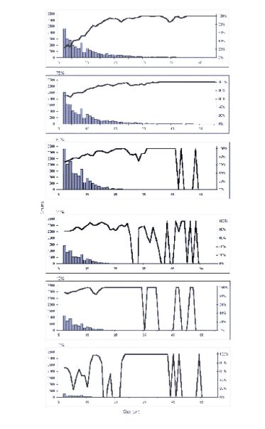 Figure 24. Size frequency distribution of natural particulates
ingested by furcilia. 100%, 75%, 50%, 25%, 10% , and 1%
refer to the percentage of ambient seawater diluted with
filtered seawater to achieve a variety of particle
concentrations. The solid line on each distribution
represents the percentage of particles in a particular size
range ingested of those particles that were available in
suspension. Note the proportion of small particles ingested
with increasing particle concentration.
Figure 24. Size frequency distribution of natural particulates
ingested by furcilia. 100%, 75%, 50%, 25%, 10% , and 1%
refer to the percentage of ambient seawater diluted with
filtered seawater to achieve a variety of particle
concentrations. The solid line on each distribution
represents the percentage of particles in a particular size
range ingested of those particles that were available in
suspension. Note the proportion of small particles ingested
with increasing particle concentration.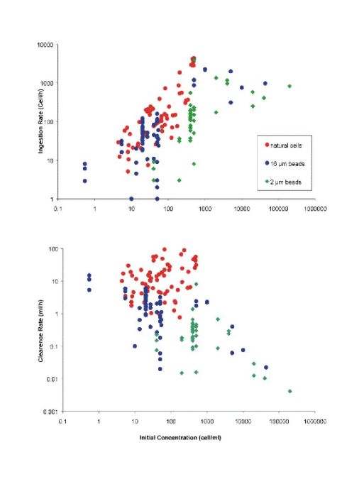 Figure 25. Ingestion and clearance rates for all experiments including those
conducted with beads and natural particulates. The functional response curve
extends over particle concentrations between 1 and 100,000 /ml. Clearance rate at
ambient concentrations typical of winter conditions (about 10 to 50/ml) was
approximately 80 ml/individual/h.
Figure 25. Ingestion and clearance rates for all experiments including those
conducted with beads and natural particulates. The functional response curve
extends over particle concentrations between 1 and 100,000 /ml. Clearance rate at
ambient concentrations typical of winter conditions (about 10 to 50/ml) was
approximately 80 ml/individual/h.
Results: Ambient concentrations (particles/ml) at t0, ingestion and clearance rates:
Treatment Concentration at t0 ingestion (part/h) clearance (ml/h)
100% 228 1506 31
75% 125 918 19
50% 176 1186 36
25% 63 424 11
10% 45 - 3
1% 16 - -
Ingestion and clearance rates could be calculated only for particle concentrations above 45/ml. This was probably because the larvae were held in surface collected water for 1 hour before the experiment and may have saturated before we began the experiment. The possibility of fecal pellet production, as examined in last year’s experiments, also exists. In general, the shape of the functional response curve was similar to that in experiment5 but without the s-shaped initial form of the Type II response. Particle size distributions were also similar to those in experiment5 along with the proportion of particles removed from suspension.
6.5.2.7 Experiment 7, 08 September 2002
Objective: To repeat the functional response experiments performed in experiment 5 and 6 with the same furcilia, but different water.
Methods: Larvae were the same as used in experiment 5 and 6. Water was collected by bucket from the dive zodiac between floes in and amongst extensive slush and melt water.
All furcilia were observed, photographed and measured after this experiment.
Results: Ambient concentrations (particles/ml) at t0, ingestion and clearance rates:
Treatment Concentration at t0 ingestion (part/h) clearance (ml/h)
100% 472 2918 15
75% 230 1450 16
50% 131 812 15
25% 58 83 2
10% 31 61 3
1% 9 - -
Again, particle concentrations were relatively low so ingestion and clearance rates were also low. The larvae seemed to be a bit ‘tired’ after going through two other experiments. Nevertheless, ingestion rates were comparable to those obtained at similar particle concentrations in experiment 5 so these data appear to be useful.
6.5.2.8 Experiment 8, 10 September 2002
Objective: To evaluate ingestion by furcilia using particle depletion over a larger concentration range.
Methods: Furcilia were collected on 9 September by Reeve net. Water was collected by bucket from the stern of the ship while en route from Station 5 to Renauld Island. Otherwise, all treatments are as in experiments 5,6, and 7.
Results: Particle concentrations were extremely low in this experiment. Ambient concentrations (particles/ml) at t0, ingestion and clearance rates are as follows:
Treatment Concentration at t0 ingestion (part/h) clearance (ml/h)
100% 77 548 14
75% 57 574 12
50% 32 - -
25% 24 45 2
10% 17 - -
1% 8 - -
Negative ingestion and clearance rates appear to be due to particle production by the furcilia. However, the 75 and 100% treatments were similar in concentration to the lowest in previous experiments.
6.5.2.9 Experiment 9, 12 September 2002
Objective: To evaluate short term particle depletion by a single furcilia.
Methods: Furcilia and water were the same as in experiment 8. A single furcilia was placed in a 200 ml flask with surface-collected water and particle concentration monitored over a 420 min time frame on a sliding time scale: 10 min intervals for the first hour, then 20 min intervals and eventually 30 min intervals.
Results: There was significant variability in the short term ingestion, so much so that it was not possible to calculate an ingestion or clearance for time points less than 60 min. If ingestion is calculated over 1 h then 1200 particles/h at a concentration of 200/ml is consistent with the results of previous experiments.
6.5.2.10 Experiment 10, 13 September 2002
Objective: To determine ingestion rates of furcilia feeding on natural particulates and beads as a tracer.
Methods: Water was collected by bucket from the surface while at anchor at Palmer Station. A sample for preservation in Lugols was collected. Furcilia were collected by Reeve net on 11 September. A bead stock solution was made to 20,000/ml. 2 ml of this was added to 2 L of bucket-collected water to give equal amounts of particles and beads. Non-invasive optical sampling was at t0, t2, and t9 h.
Results: Ambient concentrations in particles/ml at t0, ingestion and clearance rates:
Treatment Total Concentration Ingestion (part/h) Clearance (ml/h)
100% 863 1061 9
75% 372 246 3
50% 177 33 0.71
25% 67 - -
10% 21 - -
1% 9 - -
The reason for negative values in this experiment was because the control decreased quickly, so when the experimental values were corrected for the control, negative ingestion and clearance rates result. It is not known why the controls decreased so rapidly. The guts of the furcilia were packed with 16 μm beads, but the intestines contained very little. This suggests that the beads were not able to move into the intestines.
6.5.3 Overall Conclusions: There is no selection between polystyrene beads and natural particulates in either the 16 or 2 μm size category. Stage 4 and 5 furcilia appear to use a Type I (linear) functional response when they have been starved in filtered seawater for an hour or more, and a Type II (sigmoidal) functional response when they have been feeding for some period of time. This is typical of suspension feeders which require a chemical or mechanical signal for motivational feeding. When all the data for beads and natural particulates are combined for all experiments, ingestion rate increases exponentially with increasing particle concentration without saturation (Figure 25). Since krill larvae rarely, if ever, are exposed to the artificially elevated concentrations used at the upper end of these experiments, we would not expect larvae to have adapted mechanisms for dealing with such concentrations. These larvae appear to be scavengers clearing everything with a size range of 2 um to greater than 100 um in diameter. As the gut becomes full, material passes through at a rate proportional to ingestion, and no saturation is obtained.
As noted in the cruise reports for microplankton and ROV observations of furcilia distributions, there is an interesting negative relationship between the presence of furcilia and microplankton abundance. We can ask: What is the potential impact of furcilia feeding on the microplankton community across the survey grid? To address this we need three pieces of information, the relative abundance of furcilia, the abundance of microplankton in the surface waters, and the functional response of furcilia feeding on microplankton-sized particles. Furcilia abundance was highly variable and locally extremely patchy. Where furcilia were observed, they could range in concentration from 10 to tens of thousands per cubic meter making generalizations quite difficult. However, an average concentration at a site where furcilia were abundant would be reasonable at 1000/m3. Our measured ingestion and clearance rates for furcilia feeding on microplankton at abundances found during this cruise (about 10 to 100 cells/ml) is about 100 cells/individual/h and 80 ml/individual/h, respectively. The potential clearance for a furcilia population then is (.08 L/h) (24h/day) = 1.92 L/day. This potential clearance rate is sufficient to account for complete clearance of nearly twice the volume of water the furcilia are residing in. Thus the low levels of microplankton in the regions where furcilia are abundant may be the result of two factors: low growth and turn over of the microplankton community, and very high clearance rates for particles in that size range. This is good example of top down control of a prey community by a grazing population. The next step in this analysis is to establish quantitative abundances for furcilia from the ROV transect data and couple this in a simple predator-prey model of prey abundance with season and clearance by the furcilia.
6.6 Operation and use of the Simrad EK500
(Scott Gallager, Alec Scott, and Dicky Allison)
Data for the entire cruise were collected from all three frequencies on the Simrad EK500 from the 200 mile limit on day 215 and back again on day 258. There are a number of issues which need to be considered for those interested in using the Simrad data: 1. Configuration files used during collection of the data, 2. Processing of the raw data and production of Matlab files, 3. Calibration of the raw 20 log r backscatter intensity, 4. Noise produced while cruising through ice and efforts to filter the data, and 5. Correlation of events on the cruise, such as CTD and MOC1 and 10 with Simrad data. Each of these elements will be discussed briefly (additional information is included in the ships data report).
6.6.1 Configuration files. The EK500 may be set up manually through operation of buttons on the control panel, or by sending it a file from RVDS or other system controller. Details of the configuration will not be given here since they are included in the manual and in the file residing on the server. However, some information may be useful. Telegrams of 20 log r single ping data from the 38, 120, 200 kHz transducers are transmitted to RVDAS via RS232 at 115kb and logged daily. New files are started at 2000. The ping interval is set to 10 seconds since that is the minimum that can be supported at this baud rate (this really should be done through Ethernet).
6.6.2 Data processing. All processing files are included in the data CD. To process the raw simrad output, the perl script simandmwaythen.pl (written by Karen Fisher) picks up the day.dat file, which must be set by the user, loads and outputs a series of files for each frequency and time. The Matlab m file simthenplotter_2.m picks up the output from the perl script, plots and saves mat files. The m file called plotsimrad.m asks you for the Matlab filename and plots the output. All the Matlab files for each day of NBP0204 are on the data CD in gz zipped format. All the user needs to do is to unzip the mat file of choice, and run plotsimrad.m. You do not need to go back to the raw data if you just wish to plot data for a particular day or time window.
6.6.3 Calibration. There appears to be some issue surrounding the EK500 as to why it was never calibrated correctly. However, we had the opportunity on this cruise to compare the output from BIOMAPER-II directly with the EK500 on several occasions. The procedure was to crosscorrelate the two data sets for a particular time window and determine the offset for each frequency for the 20 log r backscatter intensity. The EK500 data were thus corrected by the addition of 4 db to the 38 kHz (BIOMAPER-II is actually 43 kHz), 6 db to the 120, and 4 db to the 200 kHz. In addition, the data in the *.mat files are corrected for the offset produced by the noise margin setting on the EK500 of 8 db. These corrections produced echograms of color output near equivalent to the plots produced by BIOMAPER-II while in the water at the same time. This is not a true calibration since the accuracy is unknown, but it probably gives correct backscatter intensity within a few db. The range is -100 to -40 and color scaled (thanks to Gareth Lawson) in the plots just as in the output from BIOMAPER-II Plotsimrad.m allows you to select the times within a given day to plot so you can "zoom in" on specific activities such as CTD or MOCNESS casts. We have included the perl script on the data CD if the user wishes to go back to the raw data and re-process them for some reason.
6.6.4 Noise. Extensive acoustic noise is generated as the ship moves through ice. Some effort was put into filtering ice noise with the hope that underlying data were merely obscured. However, it is clear now that when a ping is contaminated by ice noise, the underlying data is completely obliterated. In light ice about every third or fourth ping might not be contaminated so filtering out the noisy pings from the good pings is a relatively simple task. In heavy ice, however, the records became virtually unusable. Only when the ship stopped for a CTD cast or other activity were good data obtained.
6.6.5 Events. A Simrad log was established from the event log to allow association of events in decimal yearday where clean data are available in the Simrad records. This log is included in the Appendix 10 of this report and is a very handy guide for potential simrad users. Events such as 1-m MOCNESS and 10-m MOCNESS trawls, CTD casts, Tucker Trawls and Reeve net deployments are given with the associated decimal yearday to allow easy plotting of associated acoustic data.
In addition to providing the scientific party with real time acoustic data throughout the cruise, the objective of this effort was to observe the association of acoustic backscatter with thermal gradients measured with the CTD and the CMiPS high resolution temperature probe. Acoustic energy scatters off particles and plankton suspended in the water as well as relatively strong gradients in density produced by microstructure or mixing. The question is thus: When we see fine layering on the order of a few meters in thickness in acoustic records, does this represent layers of plankton and particles or physical processes such as turbulence? Two CTD casts are presented here as an example of the kind of relationship one could expect from this analysis. A Matlab script was written to display an acoustic record for a particular time window when a CTD cast was made. The user is prompted to use the mouse and draw a line next to the down cast observed on the acoustic record. The temperature data (T090c) for that cast is pulled in and depth matched to within a few centimeters with the acoustic data falling under the line. A plot is drawn of the temperature profile and the first order gradient in temperature next to the acoustic record. A scatter plot is then produced for acoustic backscatter intensity and temperature gradient. In the two examples shown here (Figure 26), backscatter ranges from –100 to –60 db along the zero axis of the temperature gradient.
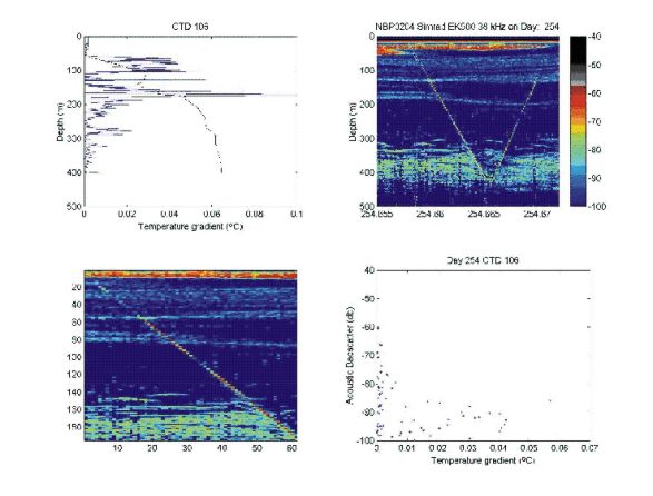 Figure 26. Multi-panel plot of EK500 38 kHz acoustic backscatter data on day 254 showing a
CTD trace, intense layering near the surface and light wispy layers down to 200 m. The white
line was drawn by the user to identify where acoustic and temperature data from the CTD are
correlated in the bottom right panel. The top left panel show the temperature profile and first
order gradient extracted from that profile.
Figure 26. Multi-panel plot of EK500 38 kHz acoustic backscatter data on day 254 showing a
CTD trace, intense layering near the surface and light wispy layers down to 200 m. The white
line was drawn by the user to identify where acoustic and temperature data from the CTD are
correlated in the bottom right panel. The top left panel show the temperature profile and first
order gradient extracted from that profile.
Backscatter also ranges from –100 to about –85 with increasing temperature gradient. Where the thermal gradient was low, the water column is most likely mixed, whereas stability increases with increasing gradient. Therefore high backscatter at low thermal gradient could be interpreted as resulting from turbulence, while high backscatter in regions of high thermal gradient may be due to plankton and particles. Without an independent measure of particulates it is impossible to differentiate the source of these signals. However, this is one of the purposes of the VPR cameras on BIOMAPER-II so we look forward to processing those data in the near future. Figure 27 gives an example of an acoustic record from the 38 kHz transducer of a krill patch (identified by the VPR cameras).
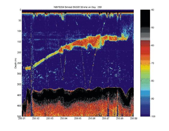 Figure 27. Krill patch intersected by the CTD on day 250.
7.0 Optical Plankton Counter and ADCP Studies of Zooplankton
(Ryan Dorland and Meng Zhou [Project PI, not present on cruise])
The objective of our research is to determine the distribution of meso- and macro-zooplankton, especially larval, juvenile, and adult krill, in relation to the mesoscale and regional circulation. Additionally, in situ rate measurements of both specific and population growth and mortality for zooplankton in the study region will be estimated from bio-volume spectra.
Circulation measurements were obtained using a 153 kHz narrowband Acoustic Doppler Current Profiler (ADCP; RD Instruments) attached to the hull of the ship. Single ping data were collected continuously throughout the cruise and displayed using software developed by Meng Zhou and Eric Firing from the University of Hawaii. Current data were processed using CODAS software developed by Eric Firing and Jules Hummon. A high resolution 5-minute ensemble average data set was maintained in addition to 15-minute and one-hour average sets. Spikes appearing in the low resolution sets often appeared as single spurious points in the high resolution set, usually attributable to ship motion not properly filtered out in preliminary processing. The data sets used during this cruise are considered a first pass and will receive more thorough processing at a later time.
The finer-scale plankton surveys were conducted using an Optical Plankton Counter (OPC; Focal Technologies) attached to a 1-m MOCNESS. The OPC gathered particle size and distribution data continuously on both the oblique and upcast portions of the MOCNESS tow. Zooplankton detected by the OPC are initially distributed into roughly 3200 size categories between 250 micrometers and 14 mm equivalent spherical diameter (ESD). The 3200 size categories are later regrouped into 50 size classes and vertically integrated into 2-m depth bins (Zhou & Huntley, 1997). Because of the relatively small intake of the OPC (2 by 25 cm2), euphausiid adults would not be sampled properly. The measurements are more representative of copepods, krill larvae, and juveniles.
The OPC was mounted on the center forward section of the MOCNESS frame and tilted at a 45 degree angle to maximize flow through the tunnel at the optimal towing angle. Flow through the OPC was calculated based both on MOCNESS flow meter readings and on a General Oceanics Digital Flowmeter attached to the OPC. The flow meter was filled with mineral oil in place of seawater before each tow to prevent freezing. The Frequency-Shift-Keyed (FSK) voltage on the OPC was lowered to 0.1 V at the start of the cruise due to low resistance on a coaxial cable. Higher voltages on the OPC caused communication failures with the MOCNESS system. The OPC was operational during 17 of the 19 MOCNESS casts (Figure 28a). During MOCNESS tow 3 at station 82, communication was lost on the upward oblique portion of the 250-m tow and not recovered. OPC data collection was aborted on Tow 14 (Station 21) due to a bad connection with the center conducting cable. A new electrical termination fixed the problem in time for the next tow.
Crystal Sound served as a staging area to test equipment and work out cross-talk problems between the MOCNESS and OPC. The first tow was conducted successfully despite heavy ice conditions. Echograms were produced and combined with MOCNESS CTD data following methods similar to Zhou et. al. (1993). The time lag between the MOCNESS CTD and the ADCP transducers was determined as a function of tow angle, horizontal velocity, and pressure (Figure 28b). OPC data showed high count densities in Crystal Sound averaging 1200 individuals/m3 below 225 m. Krill composed most of the biomass in the lower MOCNESS nets, with copepods and amphipods also present.
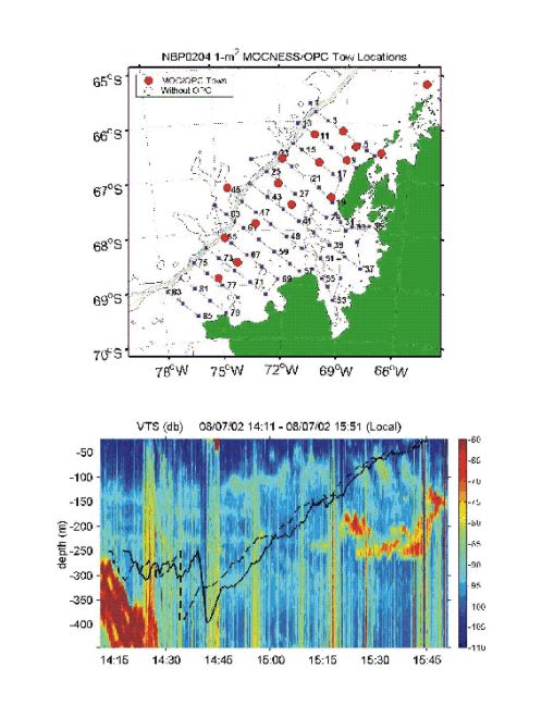 Figure 28. a) MOCNESS and OPC tow locations during NBP0204. Two tows
occurred near Renaud Island (-65 11S; -65 34W) to study vertical migration. b)
ADCP echogram for a daytime tow in Crystal Sound (-66 31.6S; -67 11.2W)
overlaid with MOCNESS pressure data plotted against both the ADCP transducer
and corrected times. A krill patch between 150 and 250 m was missed by less
than a hundred meters in the horizontal, tens of meters in the vertical. A piece of
ice caught the tow cable causing the MOCNESS to sink at 1430.
Figure 28. a) MOCNESS and OPC tow locations during NBP0204. Two tows
occurred near Renaud Island (-65 11S; -65 34W) to study vertical migration. b)
ADCP echogram for a daytime tow in Crystal Sound (-66 31.6S; -67 11.2W)
overlaid with MOCNESS pressure data plotted against both the ADCP transducer
and corrected times. A krill patch between 150 and 250 m was missed by less
than a hundred meters in the horizontal, tens of meters in the vertical. A piece of
ice caught the tow cable causing the MOCNESS to sink at 1430.
The upper nets contained little biomass. The largest krill patch observed in this region by the ADCP was between the surface and 100 m in Matha Strait (-65 46.0S; -66 46.0W). It measured over 3 km in horizontal extent. The southern section of the grid saw an increase in the number and frequency of krill patches. Over 20 km of continuous patches were observed on August 11 within the upper 150 m, ranging from several hundred meters up to two kilometers in length. The upper two nets of a MOCNESS in the area caught the edge of a 2 km patch of euphausiid juveniles. Currents in the southern section of the grid were limited to on-station times due to heavy ice. Stations near the shelf-break had uniform currents to the northeast up to 20 cm/s (Figure 29a), diminishing and becoming more variable towards Alexander Island. A weak reverse flow to the south was noticed on the closest approach to station 80, suggesting a mesoscale eddy possibly associated with larger cyclonic circulation in the inner shelf (Hoffman and Klinck 1998). Heavy ice coverage limited towing capability and reduced ADCP coverage in the central section of the survey area. Current measurements were weak and variable on-station, with exceptions of spikes in the data set coinciding with ship accelerations. On transit to Station 40 in the middle of Marguerite Bay, a 17 km krill patch was observed by the ADCP near the edge of a sea-mount. Ice conditions did not permit net tows.
Forty to fifty knot winds combined with snow forced the Palmer to drift 20 km to the south on August 30 while en-route to rendezvous with the Gould. During this twelve hour delay, current data demonstrated a velocity shear near the pycnocline (~100-120 m) with strong currents to the northeast in the surface mixed layer. The northern portion of the drift track also exhibited a barotropic component of the circulation to the northeast. Echo intensity data suggest the presence of krill within the surface layer.
The northern grid section saw a decrease in the size and frequency of zooplankton patches. Krill patches were on the order of 100 meters horizontally. Biomass from MOCNESS tows and backscattering on the echograms tended to be highter within the surface mixed layer than at depth. The Antarctic Circumpolar Current (ACC) was present at Stations 1 and 23 from ADCP current measurements. The ACC was characterized by 50 cm/s currents to the northeast along with an increase in sea-surface temperature measured by the underway flow-through system and from CTD measurements.
Two MOCNESS tows were conducted near Renaud Island to study vertical migration as part of a time-series station after the completion of survey work. The ADCP measured krill within 50 m of the surface during both tows, with only a slight decrease in layer thickness during the nighttime tow. The OPC data from the daytime tow showed a decrease in counts near the surface and around 150 m (Figure 29b). Renaud Island station contained high count densities compared to most stations in the survey region with average values between 300 to 800 individuals/m3. The biovolume spectra show a difference in slope between small and large size classes and will be used to determine the in situ rate measurements of both specific and population growth and mortality for zooplankton.I would like to thank Fred Stuart and Todd Johnson, the ETs on the N.B. Palmer for their help in resolving cross-talk problems between the MOCNESS and OPC, and to the entire BIOMAPER-II group from Wood’s Hole Oceanographic Institute (Phil Alatalo, Peter Wiebe, Dicky Allison, Scott Gallager, Gareth Lawson, and Alec Scott) for their role in MOCNESS sample collection and processing.
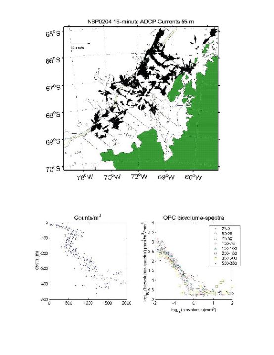 Figure 29. a) Fifteen-minute averaged ADCP currents at 55 m for NBP0204. b) OPC
count density and biovolume-spectra for each net for daytime 1-m MOCNESS tow 18
near Renaud Island.
Figure 29. a) Fifteen-minute averaged ADCP currents at 55 m for NBP0204. b) OPC
count density and biovolume-spectra for each net for daytime 1-m MOCNESS tow 18
near Renaud Island.
Hoffman, E. and Klinck, J. 1998. Hydrography and circulation of the Antarctic continental shelf: 150 E to the Greenwich meridian. The Sea, Vol. 11, 997-1042.
Zhou, M. and Huntley, M.E. 1997. Population dynamics theory of plankton based on biomass spectra. Mar. Ecol. Prog. Ser., 159, 6173.
Zhou, M., Nordhausen, W. and Huntley, M.E. 1993. ADCP measurements of the distribution and abundance of euphausiids near the Antarctic Peninsula in winter. Deep-Sea Research I., Vol. 41, No. 9, 1425-1445.
8.0 Seabird and Crabeater Seal Distribution in the Marguerite Bay Area
(Christine Ribic, and Erik Chapman)
The association of seabirds with physical oceanographic features has had a long history. For example, seabirds have been found to be associated with temperature, water masses, currents, and the ice pack. Evidence for the association of seabirds with biological features has not been as strong. Veit et al. (1993) working during the breeding season at South Georgia, was not able to find a small-scale association of seabird distributions and krill patches. Only at a very large scale was there some evidence that there were more seabirds in the vicinity of krill patches than elsewhere. This may be due to the patchiness of the krill and the inability of seabirds to track these patches at small scales. Therefore, in the Antarctic system, seabirds may associate with physical features that have a higher probability of containing krill than associating with krill patches directly. The primary objective of the seabird project is to determine the distribution of seabirds in the Marguerite Bay area and to investigate their associations with physical and biological features. A second objective is to determine the foraging ecology of the seabirds in that area.
Because the SO GLOBEC cruises took place during the non-breeding season when birds were not closely tied to breeding colonies, we hypothesized that ability to detect enhanced food resources would be the driving factor determining seabird distributions. We will be developing and testing competing models using existing knowledge of the marine system and Antarctic seabird biology. Models will be developed separately for each species or group of species based on their foraging ecology. We will be using seabird distribution and foraging ecology data that we collect along with data collected concurrently by physical and biological oceanographers to test these models. Our analysis will be extended to include other top predators, such as seals, that are recorded in sufficient numbers to allow meaningful analysis.
8.2 Methods, Data Collected, and Preliminary Results
Seabird distribution within the SO GLOBEC study area was investigated using daytime survey work, and foraging ecology of the Adelie Penguins was investigated through diet sampling. Diet sampling efforts will be used to complement an Adelie Penguin (Pygoscelis adeliae) foraging ecology study being carried out by Dr. William F. Fraser on the R/V Laurence M. Gould during the SO GLOBEC cruises. Summaries of daytime surveys and diet sampling efforts are outlined separately below. During this cruise, Crabeater Seals (Lobodon carcinophagus) were observed in sufficient numbers to comment on their abundance throughout the study area.
8.3.1 Methods: Surveys were made within a 300 m wide strip transect for birds. Surveys were conducted continuously while the ship was underway within the study area and when visibility was > 300 m. For strip transects, two observers continuously scanned a 90° area extending the transect distance (300 m and 600 m) to the side and forward along the transect line. Binoculars of 10X and 7X magnification were used to confirm species identifications. The 7X pair of binoculars also included a laser range finder. Ship-following birds were noted at first occurrence in the survey transect. Ship followers will be down-weighted in the analyses because these individuals may have been attracted to the ship from habitats at a distance from the ship. For each sighting, species, number of birds, behavior, flight direction, and any association with visible physical features, such as ice, were recorded. Distances were measured either by a range finder device as suggested by Heinneman or by the laser distance finder (when in the ice). Marine mammal sightings within the 600 m transect were also recorded. Primary ice-type and concentration within 800 m of the ship were also recorded and updated as they changed.
Surveys were conducted from an outside observation post located on the port bridge wing of the R/V NB Palmer. When it was not feasible to conduct surveys from this observation post, we surveyed from the inside port bridge wing.
8.3.2 Data Collected: Because heavy pack ice limited access to some parts of the study grid, we were unable to survey areas within Marguerite Bay and inshore along Alexander Island.
Survey Locations: See Figure 30a.
Total Survey Time: 139 hours, 42 minutes
Distance (km): 937.4 km
Boat Speed (knots): 4.5 (1.7 SD)
True Wind Speed (m/sec): 7.3 (6.6 SD)
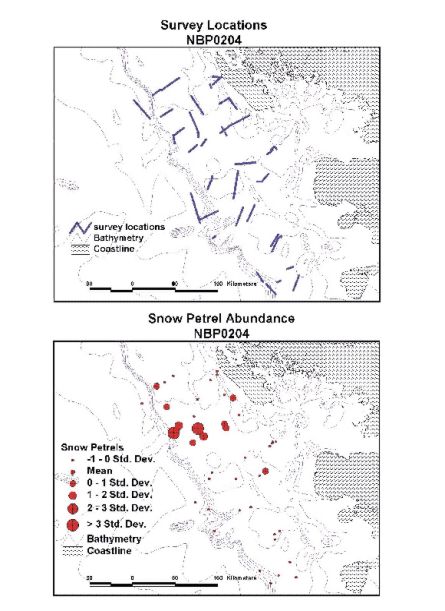 Figure 30. a) Location of top predator surveys during SO GLOBEC
IV. b) Snow Petrel relative abundance summarized for each survey
period during SO GLOBEC IV. Birds attracted to ship, or following the
ship, are down-weighted by multiplying those sightings by 0.1 in the
analysis. Values for each survey are standardized by dividing
abundance by the distance covered during the survey. Standard
deviation from the mean abundance value is associated with the mid-point of each survey location. Graduated symbols
are used to indicate
the relative abundance of birds over the study area.
Figure 30. a) Location of top predator surveys during SO GLOBEC
IV. b) Snow Petrel relative abundance summarized for each survey
period during SO GLOBEC IV. Birds attracted to ship, or following the
ship, are down-weighted by multiplying those sightings by 0.1 in the
analysis. Values for each survey are standardized by dividing
abundance by the distance covered during the survey. Standard
deviation from the mean abundance value is associated with the mid-point of each survey location. Graduated symbols
are used to indicate
the relative abundance of birds over the study area.
8.3.4.1 Ice Conditions: Ice concentrations and types varied considerably throughout the area surveyed during the cruise. The southern sector of the grid, south of Marguerite Bay and offshore of Alexander Island, was characterized by first-year, vast floes greater than 1m thick. Ice concentration varied between 8 and 10/10ths coverage here, and overall there was very little open water in this region of the grid. The central sector, offshore of Marguerite Bay, had some substantial leads several kilometers wide that were used to navigate inshore through the pack. In the central sector, the primary ice types were vast floes and large floes while ice concentration remained between 8 and 10/10ths coverage. The northern sector, north of Marguerite Bay and adjacent to Adelaide Island, had significantly lower ice-concentrations that varied between 6 and 10/10ths coverage. Surveys inshore along Adelaide Island took place within a large open water lead covered by new ice that was probably just a few days old. In general in the northern and central sectors, there was a gradient from large to small floes and cake ice moving offshore as open ocean swells were absorbed by the pack, breaking the sea-ice into smaller pieces. Offshore surveys in the northern and central sectors brought the ship within just a few kilometers of the ice-edge according to satellite ice-imagery.
8.3.4.2 Bird Observations: Overall, 915 birds from 8 species were observed during the cruise. These are similar numbers to those from the winter cruise last year (895 birds from 6 species during SO GLOBEC II). Snow Petrels, Adelie Penguins and Antarctic Petrels were the most common species observed. Crabeater Seals were also observed in relatively high abundance in the survey grid. Overall observations during SO GLOBEC IV are listed in Table 8.
Table 8. Summary of sightings during daytime survey effort within the SO GLOBEC study area during cruise NBP0204. Sightings of flying birds within the 300m transect and penguins and seals within the 600m transect are reported.
Species (common name) |
Species (scientific name) |
Number observed (NBP0204) |
Snow Petrel |
Pagodroma nivea |
488 |
Antarctic Petrel |
Thalassoica antarctica |
158 |
Southern Giant Petrel |
Macronectes giganteus |
13 |
Kelp Gull |
Larus dominicanus |
10 |
Southern Fulmar |
Fulmarus glacialoides |
8 |
Blue Petrel |
Halobaena caerulea |
1 |
Adelie Penguin |
Pygoscelis adeliae |
216 |
Emperor Penguin |
Aptenodytes forsteri |
21 |
Crabeater Seal |
Lobodon carcinophagus |
480 |
Virtually all species present in the pack ice were those adapted to foraging in ice habitat with the exception of 8 Southern Fulmars (Fulmarus glacialoides) and a single Blue Petrel (Halobaena caerulea) which are species that typically forage in open water. Results with respect to the four most common bird species, as well as Emperor Penguins and Crabeater Seals, are discussed separately below.
8.3.4.3 Snow Petrel (Pagodroma nivea): Snow Petrels were observed throughout the study area and were associated with open water within the pack-ice. Birds were observed feeding off the surface of open water both along the edges of the sea-ice and in the middle of leads. Snow Petrels were also recorded feeding between cracks in the floes and through slush and thin ice at the surface of the water. Snow Petrels were not consistent ship-followers this cruise, though they occasionally followed the ship as it cut through vast floes. In these cases, the birds were observed feeding from the exposed broken ice off the stern of the ship.
Snow Petrel abundance was similar to that observed during last winter’s cruise, but their distribution differed. Unlike during SO GLOBEC II, Snow Petrels appeared to be more abundant north of Marguerite Bay and adjacent to Adelaide Island (Figure 30b). This region was characterized by more open water, perhaps as a result of intrusions of warm Antarctic Circumpolar Deep Water here, as has been described by physical oceanographers during SO GLOBEC cruises.
.
8.3.4 4 Antarctic Petrel (Thalassoica antarctica): Antarctic Petrels have been found to be associated with the ice edge, though they range a short distance into the pack ice, feeding in open-water leads. Antarctic Petrels were also abundant during this cruise and were often found in the same areas where we recorded Snow Petrels (Figure 31a) and were also more abundant in the northern portion of the grid. In general, Antarctic Petrel abundance was much greater than that observed during SO GLOBEC II, last year’s winter cruise.
Although there are no known Antarctic Petrel breeding colonies on the Antarctic Peninsula, at-sea surveys suggest that they are present year-round in this area. As a result, bird biologists have suggested that there are colonies of Antarctic Petrels on the Antarctic Peninsula that have yet to be discovered. The Antarctic Petrels will return to their breeding colonies in about a month and their presence in the Marguerite Bay region at this time of year further supports this idea, though it is also possible that birds in this area are non-breeding adults or sub-adults.
8.3.4.5 Adelie Penguin (Pygoscelis adeliae): Adelie Penguins were observed in similar abundance to that recorded during SO GLOBEC II, last year’s winter cruise. However, unlike last year’s winter cruise, Adelie Penguins appeared to be more abundant in the northern section of the study grid, adjacent to Adelaide Island (Figure 31b). Again, this area was characterized by more open water and generally thinner ice. Adelies also appeared to be more abundant offshore, toward the ice-edge. This is where the pack was broken into small floes and cake ice by the swell from the open ocean, which may be responsible for creating the right mix of open water and ice that Adelies need for both foraging and hauling out. Biological processes associated with this area await further analysis.
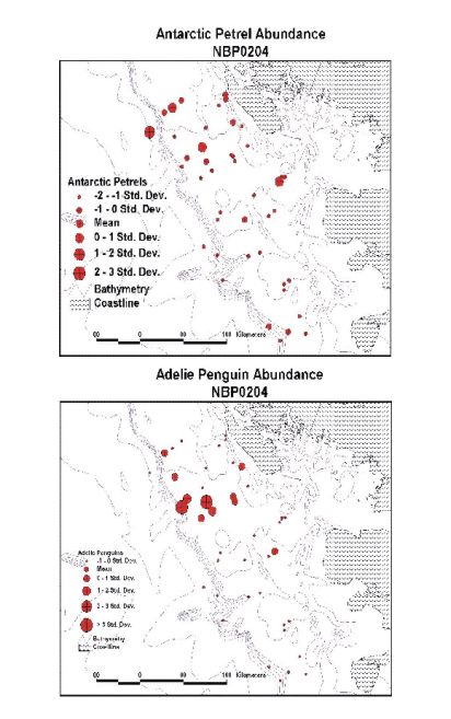 Figure 31. a) Antarctic Petrel relative abundance summarized for
each survey period during SO GLOBEC IV. Birds attracted to
ship, or following the ship, are down-weighted by multiplying
those sightings by .1 in the analysis. b) Adelie Penguin relative
abundance summarized for each survey period during SO
GLOBEC IV. (See Figure legend 30b for additional details).
Figure 31. a) Antarctic Petrel relative abundance summarized for
each survey period during SO GLOBEC IV. Birds attracted to
ship, or following the ship, are down-weighted by multiplying
those sightings by .1 in the analysis. b) Adelie Penguin relative
abundance summarized for each survey period during SO
GLOBEC IV. (See Figure legend 30b for additional details).
8.3.4.6. Emperor Penguin (Aptenodytes forsteri): Just as in the last year’s winter cruise, Emperor Penguins were recorded in the study area, but not commonly observed. In fact, the same number of birds, 21, were recorded in the study grid during this cruise as during SO GLOBEC II. Emperors Penguins are probably never common birds in Marguerite Bay, the northern extent of their breeding distribution in Antarctica. It is interesting to note that Emperor Penguins were observed in low numbers throughout the survey grid, with no obvious association with any particular section of the study area (Figure 32a).
8.3.4.7 Crabeater Seal (Lobodon carcinophagus): Many more Crabeater Seals were recorded during this cruise than during last winter’s cruise (488 during SO GLOBEC IV versus 187 during SO GLOBEC II). They appeared to be relatively abundant throughout the study grid, but were most abundant in the thicker, more concentrated ice in the southern sector of the grid (Figure 32b). Crabeater Seals feed at greater depths than other seabirds other than Emperor Penguins, and are likely tracking the availability of a prey field much deeper than other species in this survey.
8.4.1 Methods: During SO GLOBEC cruises, we opportunistically diet sampled penguins and petrels from the R/V N.B. Palmer according to protocols used by Dr. William R. Fraser. Dr. Fraser was diet sampling concurrently from the R/V L.M. Gould. We used the water off-loading technique in which birds are netted and their stomachs pumped using a small water pump . This technique is used extensively in seabird research in Antarctica [Antarctic Marine Ecosystem Research in the Ice Edge Zone (AMERIEZ), Antarctic Marine Living Resources Program (AMLR), Polar Oceans Research Group] and is preferable to methods that involve killing birds.
8.4.2 Data Collected: Three Adelie Penguins were diet sampled August 7, 2002, just off the Barcroft Islands (66°25' S, 67°10' W), south of Watkins Island and north of Adelaide Island (Figure 33). An additional 5 Adelie Penguins were diet sampled on September 3, between stations 12 and 11 (Figure 33). Digested stomach contents that were not identifiable were separated from fresh contents. Krill were identified to species and measured according to standard krill body-size measuring protocols. Data collected were turned over to Dr. William R. Fraser’s field team.
8.4.3 Preliminary Results: All birds sampled had fresh stomach contents that were easily identifiable, indicating that they had recently returned from foraging. In both locations, adult krill (Euphausia superba) comprised virtually 100% of the stomach contents. These results differ from those from Adelie diet sampling during SO GLOBEC III, when 14 diet samples, taken within a few kilometers of the first diet samples taken this cruise, revealed a diet composed of amphipods, fish, and krill. The difference in stomach contents may reflect a change in the availability of adult krill in the upper 100 m as the ice pack became established in the Crystal Sound area between SO GLOBEC cruises III and IV.
 Figure 32. a) Presence of Emperor Penguins plotted at the mid-point of each
survey period during SO GLOBEC IV. b) Crabeater Seal relative abundance
summarized for each survey period during SO GLOBEC IV. (See Figure
legend 31 b for additional detail).
Figure 32. a) Presence of Emperor Penguins plotted at the mid-point of each
survey period during SO GLOBEC IV. b) Crabeater Seal relative abundance
summarized for each survey period during SO GLOBEC IV. (See Figure
legend 31 b for additional detail). Figure 33. Locations of diet sampling efforts during SO GLOBEC IV.
The distribution of seabirds and Crabeater Seals differed during this cruise. Adelie Penguin, Antarctic Petrel, and Snow Petrel abundance were greater in the northern portion of the grid. Crabeater Seals were more abundant in the southern sector of the grid. The distribution of top predators appears to be giving a clear signal that certain areas within the grid may be sites of important processes that influence the availability of prey to predators. We look forward to future discussion and collaboration with other SO GLOBEC researchers as we investigate the link between physical and biological variables in the water column with top predator distributions during the synthesis portion of SO GLOBEC over the next several months.
Veit, R.R., Silverman, E.D. & Everson, I. (1993) Aggregation patterns of pelagic predators and their principle prey, Antarctic Krill, near South Georgia. Journal of Animal Ecology, 62, 551-564.
We would like to thank Captain Joe and all the mates for welcoming us on the bridge and putting up with having the bird box on the port bridge wing during the cruise. We would also like to thank Peter Wiebe and the other researchers on the ship for helping to schedule their work during the evenings so that we could survey for longer periods during the limited daylight available to us. Without that effort, our science would have been seriously compromised.
9.0 International Whaling Commission Cetacean Visual Survey.
(Francisco Viddi)
The International Whaling Commission (IWC) recognized that understanding environmental effects on cetaceans is important to its long-term goals. As a result, the Scientific Committee of the IWC established in 1992 a Standing Working Group on Environmental Concerns with the objective of "defining how spatial and temporal variability in the physical and biological environment influence cetacean species in order to determine those processes in the marine ecosystem which best predict long-term changes in cetacean distribution, abundance, stock structure, extent and timing of migrations and fitness". Three specific objectives were further defined under the Working Group framework as: 1) to characterize foraging behavior and movements of individual baleen whales in relation to prey characteristics and physical environment; 2) to relate distribution, abundance and biomass of baleen whale species to same for krill in a large area in a single season; and 3) to monitor interannual variability in whale distribution and abundance in relation to the physical environment and prey characteristics.
The IWC and its Working Group on Environmental Concerns recognized that these specific objectives are best addressed with a multidisciplinary ecosystem approach to data collection, analysis, and modeling. Therefore, the IWC established collaborative research programs in the Southern Ocean with the Commission for the Conservation of Antarctic Marine Living Resources (CCAMLR) and the International Global Ocean Ecosystems Dynamics (GLOBEC) program under the IWC Southern Ocean Whale Ecosystem Research (SOWER) program.
The Southern Ocean (SO GLOBEC) studies provide an ideal platform for longer term studies, where scientists from a range of disciplines can conduct intensive focused studies, within the framework of long-term data synthesis and planning. Given the shared objectives among the IWC, SO GLOBEC and CCAMLR, the IWC has determined that the most effective means of investigating these ecological issues is to focus a considerable body of cetacean research within the framework provided by these programs.
The objectives of the IWC Environmental Concerns Working Group fall within the purview of the top predator science questions developed for the SO GLOBEC program. In particular, the science question directed at understanding the winter distribution and foraging ecology of top predators in relation to the characteristics of the physical environment and the distribution and abundance of prey was of considerable interest to the IWC.
The IWC participated officially in the U.S. SO GLOBEC survey cruises in April-May 2001, August-September 2001, and April-May 2002. Participation in this, the fourth U.S. SO GLOBEC survey cruise, was through a scientist from the Instituto Antartico Chileno (INACH). The primary objectives of the cetacean scientists on these cruises were to provide a description of the abundance and distribution of whales in the SO GLOBEC study region. This will provide a census of whale distribution for a region that is little studied, especially in the austral fall and winter. Also, these data are concurrent with a suite of measurements that characterize the environment and the available prey field.
The intent of this report is to provide preliminary results from the whale observations made during the fourth U.S. SO GLOBEC survey cruise. These data, when combined with those from the three previous survey cruises, as well as with the many other data sets, will provide an unique study of cetacean habitat and foraging ecology.
Standard IWC methodology for multidisciplinary studies was used for this cruise, NBP0204. Observations of cetaceans and other predators, e.g. seals, were made from the ice tower of the RVIB Nathaniel B. Palmer, which is about 20 m above the sea level, by a single observer. Line transect sighting surveys were done throughout the daylight hours during acceptable weather conditions. Sighting effort was focused 45 degrees to port and starboard of the bow ahead of the vessel, while also scanning to cover the full 180 degrees ahead of the vessel.
During times that the ship was in sea ice, which was the majority of the time during NBP0204, the method was adjusted to include searching to the beam and behind the vessel wake, so that cetaceans and seals hidden by sea ice would be detected. A combination of eye and binocular (7x50 Fujinon) searching was used. During daylight hours, effort commenced when winds were less than 20 kts or the Beaufort Sea State was less than or equal to 5, visibility was greater than 1 mile (measured as the distance a Minke whale blow could be seen with the naked eye as judged by the observer), and the ship was actually steaming. Effort stopped while at stations or if any of the above conditions were not met. Then, only incidental observations were done. Visual observations were made along transits between stations and between transects, on transits to move the L.M. Gould to its process study sites, and on transits to move the N.B. Palmer to different areas of the study region, such as near Renaud Island and in the Gerlache Strait.
Observation effort and sightings were recorded using the laptop computer-based Wincruz Antarctic program. This program logs GPS position, ship course and speed, and a suite of environmental and sighting conditions described by the observer (Beaufort sea state, viewing conditions, weather and sea ice coverage). When possible, photographic documentation was made of each cetacean sighting for later use for individual identification, species confirmation, and habitat description.
In total 319.72 hours of observation and 152.02 hours of sighting “on effort” (“Effective effort”) (47.55 % effectiveness) were made during the entire cruise NBP0204 (Figure 34). This effort was not evenly distributed over the survey grid sections, ice coverage being the main variable affecting observation time within the study area. The total hours of incidental observations were 167.72 hours. The observation time spent within the study area totaled 264.65 hours from which 113.0 corresponded to “effective effort” (42.7 %). The average of observation hours per day was 7.61 (1.31 Standard Deviation - SD) and the average of effective effort hours per day was 3.62 (2.44 SD).
Table 9. All cetacean sightings made during U.S. SO GLOBEC survey cruise, NBP0204 (Local time +4).
GMT DATE |
GMT TIME |
Lat (̊S) |
Lon (̊W) |
SPECIES scientific name |
Group Size |
2-Aug-02 |
14:22:23 |
57.692333 |
64.121333 |
Unidentified small whale |
1 |
4-Aug-02 |
18:54:11 |
64.885833 |
64.139500 |
"like" Megaptera novaeangliae |
2 |
7-Aug-02 |
19:46:08 |
66.526333 |
67.190667 |
Balaenoptera acutorostrata |
1 |
9-Aug-02 |
20:11:46 |
67.223167 |
70.641500 |
Balaenoptera acutorostrata |
1 |
11-Aug-02 |
12:00:34 |
68.725383 |
76.106000 |
Balaenoptera acutorostrata |
3 |
11-Aug-02 |
12:12:00 |
68.735667 |
76.092333 |
Orcinus orca |
1 |
11-Aug-02 |
16:07:03 |
68.696333 |
76.158167 |
Balaenoptera acutorostrata |
3 |
11-Aug-02 |
17:19:31 |
68.682167 |
76.195167 |
Balaenoptera acutorostrata |
4 |
14-Aug-02 |
13:50:45 |
68.669000 |
76.534333 |
Balaenoptera acutorostrata |
1 |
14-Aug-02 |
15:45:52 |
68.535333 |
76.307000 |
Balaenoptera acutorostrata |
4 |
14-Aug-02 |
20:03:12 |
68.401333 |
76.138833 |
Balaenoptera acutorostrata |
2 |
14-Aug-02 |
20:34:15 |
68.380500 |
76.052833 |
Balaenoptera acutorostrata |
1 |
15-Aug-02 |
14:01:30 |
68.532833 |
74.578667 |
Balaenoptera acutorostrata |
2 |
15-Aug-02 |
17:55:24 |
68.561167 |
74.147167 |
Balaenoptera acutorostrata |
1 |
16-Aug-02 |
15:14:14 |
68.517000 |
74.176500 |
Balaenoptera acutorostrata |
1 |
16-Aug-02 |
18:31:15 |
68.454500 |
74.694833 |
Balaenoptera acutorostrata |
3 |
17-Aug-02 |
20:24:19 |
68.122833 |
74.657333 |
Balaenoptera acutorostrata |
1 |
18-Aug-02 |
16:42:52 |
67.521333 |
72.844167 |
Unidentified small whale |
2 |
18-Aug-02 |
20:13:03 |
67.590333 |
72.030833 |
Balaenoptera acutorostrata |
1 |
21-Aug-02 |
14:54:17 |
67.008500 |
73.370833 |
Unidentified whale |
1 |
21-Aug-02 |
16:13:22 |
67.048000 |
73.558500 |
Balaenoptera acutorostrata |
1 |
21-Aug-02 |
19:26:38 |
67.141500 |
74.189000 |
Balaenoptera acutorostrata |
1 |
22-Aug-02 |
23:45:00 |
67.625333 |
74.620667 |
Balaenoptera acutorostrata |
2 |
23-Aug-02 |
13:23:00 |
67.517667 |
75.097833 |
Balaenoptera acutorostrata |
1 |
23-Aug-02 |
19:21:29 |
67.508333 |
75.063833 |
Balaenoptera acutorostrata |
2 |
23-Aug-02 |
19:41:47 |
67.510667 |
75.040000 |
Balaenoptera acutorostrata |
3 |
24-Aug-02 |
13:18:27 |
67.812833 |
74.189000 |
Balaenoptera acutorostrata |
2 |
24-Aug-02 |
17:55:19 |
67.821833 |
73.998500 |
Balaenoptera acutorostrata |
1 |
24-Aug-02 |
19:41:31 |
67.800333 |
73.645000 |
Unidentified whale/dolphin |
1 |
26-Aug-02 |
14:20:26 |
68.033333 |
70.396000 |
Balaenoptera acutorostrata |
3 |
27-Aug-02 |
19:36:24 |
67.971667 |
70.732667 |
Balaenoptera acutorostrata |
1 |
2-Sep-02 |
12:10:00 |
65.620700 |
70.598167 |
Unidentified whale |
1 |
2-Sep-02 |
20:28:56 |
65.990333 |
71.116667 |
Balaenoptera acutorostrata |
1 |
3-Sep-02 |
20:24:00 |
66.227900 |
70.389833 |
Balaenoptera acutorostrata |
1 |
5-Sep-02 |
16:07:58 |
66.408500 |
71.374333 |
Balaenoptera acutorostrata |
2 |
6-Sep-02 |
21:01:00 |
66.745900 |
71.171900 |
Balaenoptera acutorostrata |
1 |
8-Sep-02 |
12:33:44 |
67.105000 |
69.247500 |
Balaenoptera acutorostrata |
1 |
8-Sep-02 |
15:23:11 |
67.048000 |
69.143667 |
Balaenoptera acutorostrata |
2 |
15-Sep-02 |
13:16:15 |
60.903333 |
63.022833 |
Unidentified Ziphiidae |
1 |
 Figure 34. Tracks where Cetacean survey took place. Blue lines represent the survey which was
made "on effort", whereas orange lines are part of the tracks where only incidental observation took
place.
Figure 34. Tracks where Cetacean survey took place. Blue lines represent the survey which was
made "on effort", whereas orange lines are part of the tracks where only incidental observation took
place.
Sighting conditions (viewing conditions) were variable during the cruise. The appropriate combination of environmental and ship conditions did not lend to long transit times for surveys “on effort”. Nevertheless, the observation and effort values accomplished in this cruise are greater than the last winter cruise, which made almost 110 hour of effort, but less than the last cruise (NBP0202) during which 183.57 effort hours were achieved.
A total of 39 cetacean sightings of 64 animals were made during the cruise (Table 9). In Antarctic waters (south of 60°S), 38 cetacean sightings of 60 animals were made. These include 31 sightings of 54 minke whales (Balaenoptera acutorostrata), 1 sighting of 2 “like” humpback whales, 1 sighting of 1 orca (Orcinus orca), 3 sightings of 4 unidentified whales, 1 sighting of 1 unidentified whale/dolphin and 1 sighting of an unidentified ziphiid and (Table 10).
All of the sightings south of 60°S, except the “like humpback whales” and the unidentified ziphiid, were from within the study area as defined by the survey grid (Figure 35a, b).
Table 10. Cetacean Sightings in Antarctic Waters (south of 60̊S)
|
Sightings |
Number of animals |
Minke Whale |
31 |
54 |
“Like” Humpback Whale |
1 |
2 |
Orca |
1 |
1 |
Unidentified ziphiid |
1 |
1 |
Unidentified Whale/Dolphin |
1 |
1 |
Unidentified Whale |
3 |
4 |
Total |
38 |
63 |
9.4 Preliminary Findings/Discussion
As stated earlier, a primary research objective of the cetacean studies within SO GLOBEC is to determine the winter distribution and foraging ecology of baleen whales in relation to the characteristics of the environment and the distribution of their prey.
In the first week of the cruise, only two sightings were made. In the Drake Passage while steaming south, a small whale was sighted, but not identified. The second sighting was made in the southern region of Gerlache Strait. Two “like” humpback whales were observed very close to shore. This sighting remained as “like” humpback whales since there was no chance to confirm species. However, surface swimming and blow patterns of these whales were like those produced by humpback whales. This becomes a very interesting sighting (if those whales were really humpbacks) due to the season (winter) of the observation. The area where these whales were seen was also an area of a very high concentration of other marine mammals (Antarctic fur seals (Arctocephalus gazella), elephant seals (Mirunga leonina) and Crabeater seals (Lobodon carcinophagus)) as well as seabirds. These observations were correlated with the vertical temperature distribution, which showed the intrusion of Circumpolar Deep Water from Drake Passage through Boyd Strait and into Bransfield Strait (CTD data).
 Figure 35. a) Distribution of all cetacean sightings in
NBP0204 in Antarctic Waters (south of 60 S). b) Distribution
of cetaceans by species observed on the NBP0204 cruise.
Figure 35. a) Distribution of all cetacean sightings in
NBP0204 in Antarctic Waters (south of 60 S). b) Distribution
of cetaceans by species observed on the NBP0204 cruise.
Only three days after the “like” humpback observation, the first Minke whale (Balaenoptera acutorostrata) was sighted (after this almost all sightings made during the cruise corresponded to Minke whales). This observation was made while work was ongoing at several stations in Crystal Sound just before entering the SO GLOBEC grid. Vertical temperature distribution in this area indicated that the trough that extends into Crystal Sound from the continental shelf was filled with Circumpolar Deep Water modified by mixing with the overlying Antarctic Surface Water. This whale was seen in a very narrow lead of open water where the ice was consistently around 9/10ths coverage. Also present was an abundant quantity of krill (mainly Thysanoessa sp. in all stages) and ctenophores at depths of 200-300 m.
The first Minke whale observed within the study area (SO GLOBEC grid) was at the limit of the northern and central sector of the grid. The animal was seen surfacing in a narrow lead of open water and once again, this observation could be correlated with the presence of Circumpolar Deep Water extending from 300 m to 500 m along the northern side of the Marguerite Trough.
The 11th and 14th of August were the best days for Minke whale sightings. Seven different sightings were made totaling 18 whales. These observations were made at the southern sector of the grid and corresponded to the southern-most sightings made during this cruise. The vertical hydrography in the area (close to station 75) showed a homogenous layer (Winter Water) and the presence of Modified Circumpolar Deep Water. The presence of this water mass indicated that no intrusions of Circumpolar Deep Water were present. The sightings on 11 August were correlated with the fact that a dense patch of “something” (probably krill) was present in the water early that morning as detected by the ADCP. These dense concentrations of potential food could explain in part the presence of whales and their high activity in the area. The BIOMAPER-II also detected an important patch of high amplitude backscatter between the surface and 150 m. In fact, one of the whales, which was spyhopping through very small cracks in the ice pack, had its mouth full of water, evidence of feeding behavior. Finally, it is important to mention that the ice coverage and thickness observed that day were not a constraint on the whales’ activity. On both the 11th and 14th , while NB Palmer was stationary (at station or assisting the Gould to set up for their process station) whales were observed blowing and spyhopping for more than 3 hours. Between the second and third Minke whale sighting, an orca was observed spyhopping not far from the baleen whales. This observation was made by one of the scientists aboard Palmer.
Four sightings of Minke whales were made during 15 and 16 August, totaling seven whales. These observation were made on the transect 10 in the southern sector of the grid. The vertical physical properties along this transect showed the presence of the southern boundary of the Antarctic Circumpolar Current. One of the sightings made on the 16th was correlated with a high number of Crabeater seals (120) along the edge of a lead of open water. During these two days, and during a BIOMAPER-II tow, very dense patches between the surface and 100 m (on 15th) and between 100 and 150 m(on 16th) were detected (this last one, one of the densest patches of backscatter seen on all four GLOBEC cruises).
Two Minke whales and one unidentified whale were sighted during 17 and 18 August. During the 17th, backscattering data collected with BIOMAPER-II varied from being low throughout most of the water column to having dense krill-like patches between 50 and 100 m.
From 21 to 24 August, 13 Minke whales were seen in 8 different sightings, while two unidentified cetaceans were also seen in two different sightings. Most of these were observed in the central sector of the grid. Whales were seen surfacing both in very wide leads of open water and in narrow small cracks in the ice pack. The results obtained from the CTD casts showed the presence of the Circumpolar Deep Water, which appeared to be moving onto the continental shelf.
A total of four Minke whale were observed in two different sightings on the 26th and 27th. The whales (3) seen on 26 August were in a wide lead of open water, while the Palmer was at station 49. Small and dense patches of acoustic backscatter located at 250 m were detected by the BIOMAPER-II in this area.
Almost a week after last sighting, two Minke whales were observed on 2 September in two different sightings. The whales and most of the seals observed during this day were seen within the same area, a pattern repeated in other occasions in this cruise. This might be a good indicator of areas rich in food resources such as krill, which is a prey item shared by both Crabeater seals and Minke whales. The vertical hydrographic structure in the area showed that the Winter Water layer was about 60 m deep. The CTD data also indicated the presence of Upper and Lower Circumpolar Deep Water. There was a considerable difference between the water column acoustic patch structure registered on 4 and 5 September. There were few patches observed on the 4th during the transects, while on the 5th there were many moderate to dense patches registered, mainly during the afternoon. The marine mammal presence (as well as the many penguin groups seen in the area) is likely associated with the existence of the dense acoustic patches.
The three whales observed on 8 September (in two different sightings) were made in a coastal polynya in the northern sector of the grid. CTD data at station 18 revealed the presence of a mixed Winter Water layer extending to 80 m. Maximum temperature observed below 300 m and its corresponding salinity were indicative of Upper Circumpolar Surface Water and Winter Water extending to the shore. Only a few krill patches were detected by the ADCP and BIOMAPER-II, but greater concentrations were observed during the afternoon.
After the sighting in Gerlache Strait where a two “like” humpback whales were seen, almost all the rest of sightings from this cruise were Minke whales (Balaenoptera acutorostrata). The average group size was 2.0 and ranged from 1 to 4 animals per group (0.965 SD). Sighting numbers of Minke whales were higher than last winter’s cruise (NBP0104) and this year’s fall cruise (NBP0202). It may confirm the last winter cruise statement, that Minke whales are the only species of baleen whale to over-winter around Marguerite Bay.
The entire study area was covered in pack ice ranging mainly between 5-10/10ths coverage, and thus, there were not many leads of open water where whales could be seen. In most cases, the whales were seen surfacing in smaller leads or cracks less than 50 m across in areas where the sea ice was not flat, but rather contained pressure ridges (this made seeing the body of a surfacing animal difficult). The entire study region was ice covered to some extent. Throughout the study region sea ice conditions varied in percent coverage as well as thickness and ice type. Even though ice coverage and thickness were greater in the southern sector, the number of sightings and whales was greater in this area. According to these preliminary data, the distribution of whales in the study area would not be absolutely limited by the ability to find open areas to breathe (although this may be an important factor for distribution - as stated in the last winter cruise report), but rather they may be limited by a combination of conditions with food resources being the key limiting factor. Brief examination of the satellite images of sea ice coverage, revealed that even in areas of complete sea ice coverage and high pressure, there appeared to be veins of open water, or at least thinner sea ice, which may offer avenues of entrance and exit for whales. It will be necessary to explore more deeply the relationship between whale distribution, abundance and activity, and ice dynamics.
As observed in the last cruises, correlation of cetacean distribution with concurrent hydrographic variables showed whales were associated with the southern boundary of the Antarctic Circumpolar Current, the frontal boundary between intrusions of warm Upper Circumpolar Deep Water and intrusion of Circumpolar Deep Water. It is important to note that the upwelling of this water mass has important effects on biological productivity due to its high nutrient content (Hofmann et al. 1996). The presence of this water mass is important to the reproductive cycle of Antarctic krill which is the prey of large populations top predators, such as penguins, seals and whales (Hoffman et al. 1996).
Cetacean sightings were particularly numerous in the southern and south-central sector of the GLOBEC grid. The correspondence between the cetacean sightings and hydrographic features suggests that the winter distribution of cetaceans along the west Antarctic Peninsula is not random, but rather is determined by the structure of the physical environment, which in turn determines prey distribution. In fact, a correlation was observed between cetacean sightings and the presence (detection) of dense krill patches. Cetacean observations were also correlated with other predator occurrence, such a crabeater seals and penguins.
The data collected during the second year of the U.S. SO GLOBEC study demonstrates that whales can be found in the Marguerite Bay area throughout the winter (as stated in the last winter cruise). Understanding the changes that occurred from the first winter cruise to the second will greatly enhance our understanding of the environmental conditions that are critical to cetacean habitat during austral winter in Marguerite Bay. Continued analyses and collection of cetacean sightings data in conjunction with concurrent prey and hydrographic distributions will allow determination of the causal relationships underlying austral winter cetacean distributions in the Antarctic Peninsula region.
Special thanks to Eileen Hofmann for all her support and ideas. Thanks to the Chief Scientist Peter Wiebe for his help and valuable comments and opinion during the entire cruise; to Erik Chapman and Baris Salihoglu for their great friendship and help in gathering data; to Bob Beardsley and Gareth Lawson for their help in mapping data. Finally, many thanks to all scientists and support staff on board for their friendship and help.
Hoffman E., Klinck J., Lascara C. and Smith D. (1996) Water mass distribution and circulation west of the Antarctic Peninsula and including Bransfield Strait. Foundation for Ecological Research West of the Antarctic Peninsula, Antarctic Research Series, 70, 61-80.
10.0 Krill Distribution, Physiology and Predations
(Kendra Daly, Kerri Scolardi, Jason Zimmerman, Emily Yam)
The overall objective of this project is to evaluate the behavioral and physiological overwintering strategies used by different life history stages of the Antarctic krill, Euphausia superba. These strategies include feeding in the water column versus on the undersurface of sea ice, herbivory, feeding on detritus, carnivory on copepods or microzooplankton (with Scott Gallager), or metabolizing body carbon and nitrogen resulting in body shrinkage. In collaboration with other projects we will construct a carbon and nitrogen budget for life history stages. Two other objectives of this project are to assess the role of ctenophores as predators on larval krill and to assess the acoustic target strength of Antarctic fishes, which are potential predators of large krill.
The first four specific objectives were assessed for larval, juvenile and adult life history stages.
1. Measure body size, dry weight, carbon, and nitrogen content.
2. Assess herbivorous and carnivorous feeding rates.
3. Measure carbon and nitrogen egestion rates.
4. Measure assimilation efficiency.
5. Measure growth and molting rates.
6. Assess the sexual maturity stage of female krill.
7. Assess abundance, distribution, and gut contents of ctenophores, determine ctenophore digestion rates, and determine ctenophore species identification using molecular techniques. We also measured respiration rates of ctenophores in collaboration with Jose Torres.
8. Measure fish parameters for input into models in order to estimate acoustic target strength.
Krill and other zooplankton were routinely collected using several types of nets and by divers for identification of species, stage, and size, for dry weight and carbon/nitrogen (CN) measurements, for physiological measurements, and for assessment of sexual maturity (Figure 36a). A Tucker Trawl was deployed at 15 stations to collect large krill. The 1.5-m2 Tucker Trawl has a ¼ in mesh graded down to a 707 μm mesh with a protected cod end. This net was usually towed in the upper 100 m for about an hour by our group. A 1-m diameter Reeve Net with a 333 μm mesh net having a 20 L protected cod end was used in tandem with a 1-m diameter Ring Net (333 μm mesh) to collect larval krill at 13 stations. The Reeve Net was hung on the 9/16” trawl wire 3 - 5 m below the Ring Net and deployed off the stern at about 10 and 15 m in depth, respectively. The propellers were run at 15-25% to keep water circulating into the nets, but with little to no forward ship movement or ice sweep-down under the hull. This method collected larval krill in excellent shape. The flowmeter readings and volume filtered for the Ring Net are shown in Table 11. Calculations for volume filtered follow the recommended equations in the General Oceanics, Inc. manual. The diving operations were done in collaboration with Jose Torres’ group at 9 sites to collect krill and ctenophores, when they were present, and to collect sea ice biota. All divers were tethered to the dive boat and therefore sampled within a 30 m radius. Sea ice biota collections were designed to sample the food available to krill feeding at the ice-water interface. Between 35 to 90 cm2 of surface area on the undersurface of sea ice was lightly scraped using a serrated tool. The loosened material was simultaneously suctioned into a sampling device. This material is usually has a lower concentration than sea ice biota higher up within ice flows. These higher concentrations, however, are not available to krill. In addition, at three ice camps we used a diaphragm pump with tubing lowered through an ice core hole to obtain samples from the ice/water interface.
Table 11. Flow meter results for the 1-m ring net from Reeve/ring net tandem deployments. G.O. Flowmeter serial # B18273
Date |
Sta |
Flowmeter Counts End |
Flowmeter Counts Start |
Counts Per Tow |
Tow Duration (min) |
Distance (m) |
Speed (cm/sec) |
Vol Filt. (m3) |
Comments |
8/29/02 |
26 |
494,914 |
468,050 |
26,864 |
65 |
722 |
18.5 |
567 |
15% turn on screws |
9/1/02 |
4 |
651,923 |
607,363 |
44,560 |
59 |
1197 |
33.8 |
940 |
ship speed 1.1 kts |
9/2/02 |
13 |
686,183 |
651,916 |
34,267 |
60 |
921 |
25.6 |
723 |
preserved sample |
9/3/02 |
11 |
719,460 |
686,175 |
33,285 |
60 |
894 |
24.8 |
702 |
|
9/5/02 |
23 |
729,744 |
719,474 |
10,270 |
60 |
276 |
7.7 |
217 |
ship speed 0.5 kts |
9/6/02 |
21 |
747,676 |
729,744 |
17,932 |
64 |
482 |
12.5 |
378 |
Strong current, nets tending under ship, props @25% |
9/7/02 |
19 |
801,648 |
747,681 |
53,967 |
63 |
1450 |
38.4 |
1138 |
Polynya, ship speed @ 0.9-1 kt |
9/8/02 |
17 |
835,917 |
801,464 |
34,453 |
60 |
926 |
25.7 |
727 |
props @ 15%, ring net bridle very twisted |
9/9/02 |
5 |
889,065 |
835,935 |
53,130 |
70 |
1428 |
34.0 |
1121 |
props @ 20%, ship speed 0.5 kts, ring net bridle very twisted; preserved sample |
9/11/02 |
RI* |
912,845 |
889,082 |
23,763 |
45 |
639 |
23.7 |
501 |
props @ 15%, ring net bridle very twisted |
*Renaud Island |
|||||||||
We were not able to use the Hydroacoustic Technology Inc. (HTI) system during net deployments, when BIOMAPER-II was on deck, due to heavy sea ice conditions. However, this system was deployed with the ship drifting in small leads in Crystal Sound and at a location about mid-shelf, and in Arthur Harbor at Palmer Station. An extensive in situ field calibration using a standard 38.1 mm diameter tungsten carbide sphere was completed to better understand changes in system efficiency observed in cold high latitude waters.
Chlorophyll a and POC and PON concentrations in the water column and in under-ice samples will be used as a measure of food available to krill. Three samples of sea ice biota were collected by divers in areas where larval krill were feeding at the sea ice interface at two stations. At all other locations where krill were not present, sea ice biota sampling sites were chosen based on ice color and type. Samples of surface ice slush/brash, where larvae are sometimes observed to feed, also were collected at every dive site. One sea ice biota sample was analyzed for chlorophyll a aboard ship and the second sample will be analyzed for particulate organic carbon (POC) and nitrogen (PON) concentrations after returning to the lab. The third sample will be analyzed by Scott Gallager for microbial identification and abundance. Chlorophyll and POC/N concentrations in size fractions (0.7 – 1, 1 - 5, 5 - 20, and > 20 μm) will be determined for surface ice slush samples and some water column samples. The ice/water interface samples collected from ice camps also will be analyzed for chlorophyll and POC/N concentrations. In addition, we collected surface seawater (intake ca. 2 m depth) at 9AM, 3PM, and 9PM from the ship’s flow- through system to correlate the fluorescence voltage output with chlorophyll concentration.
Feeding rates of krill were determined by gut fluorescence and carnivory container experiments using standard methods. Adult experimental chambers were 20 L and larval chambers were 1.5 to 3 L. Larval krill feeding on microplankton will be assessed in collaboration with Scott Gallager. Growth rates were determined by measuring the total length of a molted individual, and then measuring the length of the uropod and the telson on a molt and the recently molted krill. The larval stage also was noted for the molt and the krill to assess development. Molting rates were determined by holding approximately 100 krill for 3 to 5 days and checking for molts every 12 hours. During the GLOBEC IV cruise we completed 6 ingestion, 8 egestion, 7 assimilation efficiency, 6 growth and molting, 2 additional molting, and 4 copepod predation rate experiments. In addition 184 juvenile and adult krill from Crystal Sound and Station 75 were measured for total length and eye diameter as a continuation of a collaboration with Roger Harvey to investigate potential winter shrinkage in krill size. Carbon/nitrogen budgets will be estimated from growth, molting, and egestion rates and assimilation efficiency for different life history stages. Respiration rates measured by Jose Torres and excretion rates measured in collaboration with Kent Fanning will be used to complete the budget analyses. The results of these measurements will be assessed in relation to the abundance and distribution of different life history stages and environmental factors to evaluate overwintering strategies of krill.
 Figure 36. A. Station locations for Tucker Trawls (circles), Reeve/ring nets
(triangles), dive (diamond), and ice station (squares) collections for the Krill
Distribution, Physiology, and Predation Project. B. Relative abundance and
distribution of Euphausia superba larvae based on Tucker Trawl and
Reeve/ring net hauls and diver observations. Red circles are > 100 larvae,
black circles are 1 - 100 larvae, and yellow circles are no larvae.
Figure 36. A. Station locations for Tucker Trawls (circles), Reeve/ring nets
(triangles), dive (diamond), and ice station (squares) collections for the Krill
Distribution, Physiology, and Predation Project. B. Relative abundance and
distribution of Euphausia superba larvae based on Tucker Trawl and
Reeve/ring net hauls and diver observations. Red circles are > 100 larvae,
black circles are 1 - 100 larvae, and yellow circles are no larvae.
Several dominant species of fish, Electrona antarctica, Bathylagus antarcticus, and Gymnoscopelus nicholsi, were measured for body shape, volume, and density to investigate acoustic target strength properties of these potentially important predators on krill. Previous target strength measurements of tethered fish made on earlier GLOBEC cruises are similar to those predicted by our ongoing modeling investigation.
We have tentatively identified the dominant ctenophore present in Marguerite Bay as Callianira antarctica. Genetic samples were collected and will be analyzed by George Matsumoto (MBARI) to positively identify this species. Ctenophore abundance and distribution were determined from 28 Tucker Trawls, 8 Reeve/Ring nets deployments, 6 1-m MOCNESS and 11 10-m MOCNESS tows. Since ctenophores dissolve in preserved samples, we immediately pulled individuals out of net hauls as soon as they came on deck. Ctenophores also were collected during dives when they were present. More than 150 individuals were measured and evaluated for morphology and gut contents. Some individuals were frozen for lipid analyses along with potential prey to identify ctenophore food sources in absence of identifiable gut contents. Lipid samples will be analyzed in collaboration with Rodger Harvey. In addition we measured respiration and excretion rates for 16 ctenophores (with Jose Torres) and 20 digestion times for different prey type and number.
10.4.1 Abundance and Distribution - During the April-May cruise (GLOBEC III), few larval krill were observed anywhere on the shelf in the vicinity of Marguerite Bay. Similarly, during this follow on cruise, larval krill abundance remained low compared to that observed last year. Figure 36b shows the relative abundance of larvae based on our net tows and dive observations. No larvae were observed in Crystal Sound. In the southern part of the survey area larvae were only collected at a few locations and in very low abundance. These individuals were Furcilia stages 4 - 6 and 7.5 to 10.5 mm in length. Some larvae were collected in net hauls at stations near the mouth of Marguerite Bay. Larval krill were more prevalent in the northern end of the survey area. Tow-yowing the Tucker Trawl in the upper 15-25 m yielded more larvae than deeper tows, but they were often damaged by ice filling the net. Consequently at the northern end of the grid we switched to using the tandem Reeve/Ring net deployments in the upper 15 m. Using these nets, we collected one hundred to several hundred larvae during ca. 60 min deployments near stations 4, 13, 17, and 26. Krill larvae were Furcilia stages 4 – 6 and 8.5 to 13 mm in length. Ctenophores were present in every net tow. Larval, juvenile, and some adult E. crystallorophias also were collected at stations 81, 26, 4, 13, 11, and 17.
The furcilia at the southern stations seemed to be somewhat smaller (mode, 8 mm) with a higher proportion of individuals in the youngest stage (F4, 19%) than the northern stations larvae (mode, 10 mm; F4, 13 %) (n = 299). Nevertheless, the size and stage distribution of all larvae combined showed that the majority of furcilia were an F6 and 11 mm in length (Figure 37a), the same dominant size and stage observed last winter.
In contrast to larvae, juvenile krill (15 - 39 mm) were abundant and occurred throughout the study area. The smallest juveniles (< 20 mm) are probably early recruits from the 2002 larval stock. Juveniles larger than about 20 mm likely resulted from last year’s highly abundant larvae, which successfully overwintered and recruited to the juvenile stage last austral spring. Adult krill also were widely distributed throughout the study area compared to those collected in net tows last winter (2001). Adults were either immature females or males, 29 to 56 mm in length. Large numbers of juveniles and adults were collected by Tucker Trawls in near-surface layers (varying within the upper 100m) in Crystal Sound and in the southern region (e.g., Station 75). Towards the end of the cruise in the northern region, juveniles formed large aggregations near the surface at some locations, e.g., Station 23 and Renaud Island.
Other zooplankton collected in net tows included the euphausiids, Thysanoessa macrura (in most tow at low densities), E. crystallorophias, and E. triacantha. E. crystallorophias is typically found near shore, but occurred on the outer shelf in the northern region during this cruise. E. tricantha is typically found off-shelf below 200 m in Circumpolar Deep Water (CDW); however, numerous individuals were observed at several stations (e.g., Station 72) in areas where the CDW had flooded onto the shelf. Other common zooplankton were ctenophores, the copepods, Calanus propinquus, Metridia gerlachei, and Paraeuchaeta spp, ostracods, pteropods, amphipods, salps in the northern region, and chaetognaths. Large adult C. propinquus (> 4 mm) were particularly abundant in the northern region near the surface.
10.4.2 Food availability – Chlorophyll concentrations were very low in the water column (≤ 0.08 µg Chl L-1, Table 12) similar to concentrations observed last winter. Size fractionations indicate that 21-32 % of the total pigment (chlorophyll + phaeopigment) was > 20 µm in size, which large krill are more likely to ingest. Pigment maxima were usually in the smallest (0.7 to 1 μm) size fraction. Chlorophyll concentrations in water collected from the flow-through fluorometer three times per day ranged from 0.026 to 0.220 μg L-1, with a mean (+ 1 SD) of 0.059 + 0.050 μg L-1 (n= 117). Food concentrations also were generally low on the under surface of sea ice, in surface ice slush, and from the ice-water interface below sea ice (Table 13), and similar to last winter’s sea ice biota concentrations. Some under-ice samples had an order of magnitude higher chlorophyll concentrations (e.g., up to 0.33 μg L-1), but this is still a relatively low autotrophic biomass. Ice “food” differed from the water column in that size fractions of sea ice biota indicated that the highest chlorophyll concentrations were usually in the 5 – 20 μm size range. In both the water column and under sea ice phaeopigments concentrations accounted for 18 – 75% of the total pigment, suggesting that much of the autotrophic biomass was detrital. Heterotrophic microplankton biomass also was low (S. Gallager, personal communication) in the water column and in sea ice samples, until the last few stations in the northern region of the study area.
 Figure 37. a) Length-frequency distribution of Euphausia superba during
August-September 2002. b) Examples of adult Euphausia superba gut
and hepatopancreas for feeding and rarely feeding individuals. A) winter
krill collected in situ with pale greenish, small hepatopancreas and no
material in gut or intestine; B) winter krill after feeding on copepods
showing orange material in gut and intestine with a whitish enlarged
hepatopancreas; C) fall actively feeding krill collected in situ with dark
green gut and enlarged green hepatopancreas; D) same individual after 3
weeks of starvation showing decrease in hepatopancreas size and color.
Figure 37. a) Length-frequency distribution of Euphausia superba during
August-September 2002. b) Examples of adult Euphausia superba gut
and hepatopancreas for feeding and rarely feeding individuals. A) winter
krill collected in situ with pale greenish, small hepatopancreas and no
material in gut or intestine; B) winter krill after feeding on copepods
showing orange material in gut and intestine with a whitish enlarged
hepatopancreas; C) fall actively feeding krill collected in situ with dark
green gut and enlarged green hepatopancreas; D) same individual after 3
weeks of starvation showing decrease in hepatopancreas size and color.
Although food for larvae appeared to be very limited in the water column, copepods were very abundant at some depths and could have provided a food source for large krill.
Mature female and male and stage Vs of the large calanoid copepod, C. propinquus, were very abundant near the surface where larval krill were found. These copepods, typically > 5 mm in length, were not eaten by adult krill in experiments and thus may avoid predation due to their large size. However, given the densities of these copepods, they may compete with larval krill for scarce resources in near surface waters.
Table 12. Water column food availability for Euphausia superba as indicated by chlorophyll a (Chl a), phaeopigment (Phaeo), and total chlorophyll pigment (Chl+Phaeo) concentrations (μg L-1)
Date |
Station |
Depth |
Size fraction (µm) |
Chl A |
Phaeo |
Chl+Phaeo |
% Phaeo |
08/12/02 |
Station 75 |
190 m, fluorescence peak mid-thermocline |
>20 |
0.002 |
0.001 |
0.003 |
32.0 |
|
|
|
5 - 20 |
0.000 |
0.000 |
0.000 |
71.5 |
|
|
|
1 - 5 |
0.001 |
0.002 |
0.003 |
74.9 |
|
|
|
0.7 - 1 |
0.005 |
0.004 |
0.008 |
45.6 |
|
|
|
SUM |
0.007 |
0.007 |
0.014 |
|
|
|
|
|
|
|
|
|
08/29/02 |
Station 26 |
2 m |
>20 |
0.008 |
0.005 |
0.013 |
36.5 |
|
|
|
5 - 20 |
0.006 |
0.005 |
0.011 |
46.6 |
|
|
|
1 - 5 |
0.003 |
0.003 |
0.007 |
47.0 |
|
|
|
0.7 - 1 |
0.008 |
0.003 |
0.011 |
27.9 |
|
|
|
SUM |
0.025 |
0.016 |
0.041 |
|
|
|
|
|
|
|
|
|
09/03/02 |
Station 11 |
37 m, fluorescence peak |
>20 |
0.012 |
0.009 |
0.021 |
44.0 |
|
|
|
5 - 20 |
0.011 |
0.007 |
0.018 |
40.7 |
|
|
|
1 - 5 |
0.011 |
0.005 |
0.016 |
28.6 |
|
|
|
0.7 - 1 |
0.019 |
0.006 |
0.025 |
25.6 |
|
|
|
SUM |
0.053 |
0.028 |
0.080 |
|
|
|
|
|
|
|
|
|
09/03/02 |
Station 11 |
290 m, fluorescence peak |
|
0.003 |
0.011 |
0.014 |
78.787 |
|
|
|
|
|
|
|
|
09/03/02 |
Station 11 |
405 m, fluorescence peak |
|
0.002 |
0.014 |
0.015 |
87.837 |
10.4.3 Physiological Measurements – Final analyses of the feeding experiments have not been completed; however, several lines of evidence indicate that most adult E. superba were rarely feeding in situ. Almost all adults collected had very little material in their gut, rarely any in their intestine, and their hepatopancreas was small and almost colorless to pale green. Gut fluorescence, a relative indicator of herbivory, was 2 to 5 times lower (0.4 ng pigment per krill) in winter adults than values obtained during the previous fall cruise for adults (90 ng - 15 μg pigment per krill), and 1 to 2 times lower than values obtained for adults (5 – 28 ng per krill) during last winter (2001). Given the low chlorophyll values in the water column it is not surprising that adults may not have fed on phytoplankton. However, adults also did not appear to be feeding on copepods, the dominant heterotrophic food source available. Preliminary evidence from net hauls and the Video Plankton Recorder (VPR) cameras (S. Gallager, personal communication) indicates that the vertical distribution of adults and potential copepod prey overlapped in some locations, especially after dark. When offered copepods in feeding experiments some krill fed readily (3 out of 10), while the remainder did not feed at all. Adults that did feed showed a preference for calanoids < 5 mm and Metridia, but avoided Paraeuchaeta. The individuals that did ingest copepods showed evidence of feeding within 8 hours (overnight) with whitish material in their gut and an enlarged and whitish hepatopancreas. None of the adults collected in situ showed similar features (Figure 37b).
Table 13. Under-ice food availability for Euphausia superba as indicated by chlorophyll a (Chl a), phaeopigment (Phaeo), and total chlorophyll pigment (Chl+Phaeo) concentration (μg L-1) of sea ice biota. Under-ice samples were simultaneously scraped and suctioned from the ice interface by divers using a sampling device. The ice station samples were collected using a diaphragm pump with tubing lowered through an ice core hole.
Date |
Station/Event |
Sample |
Size Fraction (µm) |
Chl a |
Phaeo |
Chl+Phaeo |
% Phaeo |
8/5/02 |
Crystal Sound, Dive #1 |
Under-ice surface |
|
0.035 |
0.026 |
0.062 |
42.8 |
8/6/02 |
Crystal Sound, Ice Station |
Under-ice-water interface |
>20 |
0.001 |
0.001 |
0.003 |
44.7 |
|
|
|
5 - 20 |
0.012 |
0.008 |
0.020 |
38.6 |
|
|
|
1 - 5 |
0.003 |
0.002 |
0.005 |
40.8 |
|
|
|
0.7 - 1 |
0.006 |
0.003 |
0.008 |
34.6 |
|
|
|
SUM |
0.022 |
0.014 |
0.036 |
|
8/9/02 |
Ice Station |
Under-ice water interface |
>20 |
0.031 |
0.007 |
0.038 |
18.3 |
|
-67 13.35 S, -70 38.69 W |
|
5 - 20 |
0.026 |
0.020 |
0.047 |
43.4 |
|
|
|
1 - 5 |
0.006 |
0.003 |
0.008 |
31.0 |
|
|
|
0.7 - 1 |
0.010 |
0.003 |
0.013 |
24.3 |
|
|
|
SUM |
0.073 |
0.033 |
0.106 |
|
8/12/02 |
77, Dive # 2 |
Under-ice surface |
|
0.061 |
0.047 |
0.108 |
43.2 |
8/16/02 |
67, Dive # 3 |
Under-ice surface |
|
0.030 |
0.031 |
0.061 |
51.2 |
8/16/02 |
67, Dive # 3 |
Surface ice slush |
>20 |
0.007 |
0.001 |
0.008 |
15.2 |
|
|
|
5 - 20 |
0.028 |
0.012 |
0.040 |
29.5 |
|
|
|
1 - 5 |
0.009 |
0.003 |
0.012 |
24.5 |
|
|
|
0.7 - 1 |
0.014 |
0.004 |
0.018 |
22.6 |
|
|
|
SUM |
0.058 |
0.020 |
0.078 |
|
8/24/02 |
62, Ice Station |
Under-ice water interface |
>20 |
0.002 |
0.001 |
0.003 |
27.0 |
|
|
|
5 - 20 |
0.006 |
0.009 |
0.015 |
59.2 |
|
|
|
1 - 5 |
0.003 |
0.001 |
0.004 |
36.0 |
|
|
|
0.7 - 1 |
0.005 |
0.003 |
0.008 |
33.1 |
|
|
|
SUM |
0.016 |
0.014 |
0.030 |
|
8/26/02 |
40, Dive # 4 |
Under-ice surface |
|
0.072 |
0.040 |
0.112 |
35.7 |
8/29/02 |
26, Dive # 5 |
Under-ice surface |
|
0.141 |
0.104 |
0.245 |
42.4 |
8/29/02 |
26, Dive # 5 |
Surface ice slush |
>20 |
0.035 |
0.006 |
0.041 |
15.3 |
|
|
|
5 - 20 |
0.088 |
0.020 |
0.108 |
18.6 |
|
|
|
1 - 5 |
0.022 |
0.003 |
0.025 |
10.8 |
|
|
|
0.7 - 1 |
0.032 |
0.005 |
0.037 |
13.7 |
|
|
|
SUM |
0.177 |
0.034 |
0.211 |
|
9/4/02 |
16, Dive # 6 |
Under-ice surface |
|
0.210 |
0.045 |
0.256 |
17.7 |
9/4/02 |
16, Dive # 6 |
Surface ice slush |
>20 |
0.016 |
0.004 |
0.020 |
18.8 |
|
|
|
5 - 20 |
0.032 |
0.010 |
0.042 |
24.6 |
|
|
|
1 - 5 |
0.011 |
0.004 |
0.015 |
25.2 |
|
|
|
0.7 - 1 |
0.015 |
0.004 |
0.019 |
20.0 |
|
|
|
SUM |
0.074 |
0.022 |
0.095 |
|
8/8/02 |
14, Dive # 7 |
Under-ice surface |
|
0.096 |
0.031 |
0.126 |
24.4 |
9/5/02 |
14, Dive # 7 |
Surface ice slush |
>20 |
0.025 |
0.004 |
0.028 |
13.6 |
|
|
|
5 - 20 |
0.056 |
0.010 |
0.066 |
14.7 |
|
|
|
1 - 5 |
0.039 |
0.006 |
0.045 |
13.5 |
|
|
|
0.7 - 1 |
0.046 |
0.007 |
0.053 |
14.0 |
|
|
|
SUM |
0.166 |
0.027 |
0.193 |
|
9/8/02 |
17, Dive # 8 |
Under-ice surface |
|
0.051 |
0.017 |
0.067 |
24.8 |
9/8/02 |
17, Dive # 8 |
Surface ice slush |
>20 |
0.043 |
0.007 |
0.050 |
14.2 |
|
|
|
5 - 20 |
0.080 |
0.013 |
0.093 |
13.9 |
|
|
|
1 - 5 |
0.021 |
0.005 |
0.026 |
20.1 |
|
|
|
0.7 - 1 |
0.072 |
0.000 |
0.064 |
0.0 |
|
|
|
SUM |
0.216 |
0.025 |
0.233 |
|
9/11/02 |
Renaud Island, Dive #9 |
Under-ice surface |
|
3.140 |
0.410 |
3.549 |
11.5 |
|
|
|
>20 |
0.065 |
0.022 |
0.087 |
24.8 |
9/11/02 |
Renaud Island, Dive #9 |
Surface ice slush |
5 |
0.074 |
0.002 |
0.075 |
2.6 |
|
|
|
1 |
0.019 |
0.004 |
0.023 |
19.5 |
|
|
|
0.7 |
0.170 |
0.000 |
0.153 |
0.0 |
|
|
|
SUM SF |
0.328 |
0.010 |
0.338 |
|
Larval and juvenile krill appeared to feed more opportunistically. Juvenile gut fluorescence values ranged from 0.4 to 70.8 ng pigment per individual compared to values during the fall of 6 to 234 ng per individual. Larvae varied from 0.25 - 75.7 ng pigment per individual and almost all had whitish material in their gut and intestine when collected. These winter values are similar to larval gut fluorescence (0.8 – 7.4 ng per individual) during last winter (2001). The tandem nets near surface collected detrital material and small plankton, which may have provided some food for larvae and juveniles. This material consisted of radiolarians and mats of diatoms with long setae remaining from the fall bloom. Numerous veliger larvae, gastropods, small pteropods, foraminifera, and trochophore larvae also were stuck to these aggregates probably from turbulence in the nets.
Euphausiids are obligate molters. When they do molt they may increase or decrease in length. Molting experiments indicated that larvae molted about every 40 to 60 days, juveniles about every 29 to 62 days, and adults molted about every 28 to 36 days. The shortest molting periods for larvae and juveniles occurred at the end of the study in early-September. On average there was no growth evident among individuals that molted during most of the study period, except for the early September larvae and juveniles which showed a 4.25 and 2.36 % increase in uropod length, respectively. The estimated growth rates for these individuals are 0.013 mm d-1 for larvae and 0.015 mm d-1 for juveniles. Not only were growth rates minimal for most of the study period, but 76% of the furcilia that molted displayed arrested development. The low growth rates and lack of development to the next life history stage suggest that larvae were food limited during winter 2002. The measurable growth rates for larvae and juveniles in September suggests an increase in food availability during this early spring period. Larvae apparently put additional resources towards increasing length before developing to the next stage.
Larval krill had a highly patchy distribution and were relatively low in abundance during both the fall and winter cruises compared to abundances last year. Reproductive success apparently was high during summer 2000-2001 and relatively low during summer 2001-2002. Alternatively, reproduction may have been relatively high last summer, but fewer larvae were advected onto the shelf. Larvae appeared to inhabit the upper 25 m of the water column, but were seldom seen feeding directly on the undersurface of ice floes until early September in the northern end of the study area. The high densities of late stage C. propinquus may compete with larval krill for scare resources near surface.
Juveniles were very abundant in contrast to the total lack of juveniles last year. The vertical and horizontal distribution of adults appeared to differ from the patterns observed last winter in that they were more widely distributed and formed large layers in the upper 100 m in some locations during this study.
Food availability in the water column and under sea ice was generally low and similar to last year. Thus the early formation of sea ice in this region does not necessarily guarantee that sea ice biota will be a significant food resource during winter. Particulate organic matter and detritus may have been more concentrated near the ice/water interface, but those samples remain to be analyzed. Although large concentrations of copepods were present in the water column, adult krill did not appear to be actively feeding on them.
The relatively long intermolt period and the lack of growth and development by all stages indicates that krill were food limited, particularly during August.
11.0 Fish and krill ecology/ krill physiology
(Jose Torres, Joe Donnelly, Melanie Parker, Tom Bailey)
The objectives of our program were three-fold. The first was to describe the distribution and abundance of larger size classes of krill and micronektonic species likely to prey on krill, primarily fishes. The second was to describe the distribution and abundance of krill larvae underneath sea ice at various locations within the survey grid, to collect larvae for physiological manipulation, and to collect samples of the under-ice surface to assess food availability for larval krill. Our second objective was a collaborative effort with the K. Daly program. The third objective was to describe the respiration, excretion, and physiological condition of all size classes of krill within the survey area, and to make similar measurements on other important micronektonic and zooplanktonic species as opportunities arose.
11.2.1 Fish and large krill (micronekton) abundance
Micronekton was sampled using a 10 square-meter mouth area, Multiple Opening Closing Net and Environmental Sensing System (MOCNESS) equipped with 3 mm mesh nets and towed at a speed of 1.5 to 2 knots, ice conditions permitting. Vertical strata sampled during the course of the survey depended on bottom depth. For stations greater than 1000 m in depth, strata sampled were: 1000-500 m, 500-200 m, 200-100 m, 100-50 m, 50-0 m. For stations greater than 500 m in depth, depth strata sampled were 500-300 m, 300-200 m, 200-100 m, 100-50 m, 50-0 m. Sample depths for shallower bottoms were adjusted to make best use of the 5 sample nets. MOC 10 samples were collected at the survey stations listed in Table 14.
Table 14. Station locations and positions of 10-m MOCNESS tows taken on NBP0204.
Trawl number |
station number |
start location |
end location |
m10-001 |
cs-4 |
66 32.544 S; 67 05.818 W |
66 35.854 S; 67 08.169 W |
m10-002 |
75 |
68 39.957 S; 76 08.852 W |
68 42.847 S; 76 01.211 W |
m10-003 |
72 |
68 34.368 S; 74 09.035 W |
68 35.522 S; 74 05.219 W |
m10-004 |
65 |
68 08.814 S; 74 35.499 W |
68 07.654 S; 74 39.359 W |
m10-006 |
44 |
67 09.236 S; 73 14.654 W |
67 02.381 S; 73 21.162 W |
m10-007 |
between 62 and 48 |
67 53.216 S; 73 05.875 W |
67 54.625 S; 73 02.111 W |
m10-009 |
13 |
67 57.160 S; 71 02.845 W |
66 04.590 S; 71 16.730 W |
m10-010 |
22 |
66 49.243 S; 71 25.277 W |
66 53.084 S; 71 25.547 W |
m10-011 |
19 |
67 28.010 S; 69 32.084 W |
67 23.399 S; 69 32.719 W |
11.2.2 Under-ice abundance of krill larvae
Krill furcilia were sampled underneath pack ice using SCUBA (Figure 38a, b) at the stations listed in Table 15. To observe and collect the marine life that inhabits the under-ice environment SCUBA diving is a reliable and effective method. Furcilia concentrations were estimated using videography along a 10 m transect line anchored at each end with ice screws. When present, furcilia were collected with hand-held nets for physiological manipulation. Microbiota under the under-ice surface was sampled using a suction collector (see K. Daly narrative). Standard blue water diving techniques adapted for extreme cold water and overhead ice cover as described below were used to maximize diver safety.
Diving beneath the pack ice requires a considerable amount of preparation and specialized equipment. First, to deal with the ice cold water, a dry suit is required. A dry suit is basically a tough rubber suit with a valve to inflate it and a valve to let the air out. It is made with feet attached, so that the only parts of your body that stick out are your head and your hands. Tight rubber seals at the neck and wrists prevent water from entering the suit. Because it is dry, you can wear heavy underwear underneath the suit to protect you from the cold. A tight rubber hood and protective gloves complete the Antarctic SCUBA diving outer garments. The suit attaches to your compressed air bottle via a pressure hose to allow inflation.
 Figure 38. a) Divers Kerri Scolardi and Melanie Parker using nets used to
capture furcilia. Note the tethers. Photo by Stian Alessandrini. b) The
NBP0204 dive team. Left to right: Melanie Parker, Stian Alessadrini, Jose
Torres, and Kerri Scolardi. Photo by Sarah Dizik.
Figure 38. a) Divers Kerri Scolardi and Melanie Parker using nets used to
capture furcilia. Note the tethers. Photo by Stian Alessandrini. b) The
NBP0204 dive team. Left to right: Melanie Parker, Stian Alessadrini, Jose
Torres, and Kerri Scolardi. Photo by Sarah Dizik.
Table 15. Station locations and positions of under-ice SCUBA dives on NBP0204.
Dive number |
station number |
location |
divers |
date |
1 |
CS-4 |
66 31.370 S; 67 16.150 W |
KS, MP,SA |
5-Aug |
2 |
77 |
68 53.866 S; 75 08.425 W |
JT, KS, SA |
12-Aug |
3 |
66/67 |
68 26.542 S; 74 45.712 W |
JT, MP,SA |
16-Aug |
4 |
40 |
68 02.000 S; 70 23.960 W |
KS, MP,SA |
26-Aug |
5 |
26 |
67 08.036S; 72 09.176 W |
JT, KS, SA |
29-Aug |
6 |
16 |
66 44.800 S; 70 10.290 W |
JT,KS, SA |
4-Sep |
7 |
14 |
66 23.689 S; 71 21.476 W |
KS, MP,SA |
5-Sep |
8 |
17 |
66 56.913 S; 69 30.439 W |
KS, MP,SA |
8-Sep |
9 |
RI-2 |
65 09.660 S; 65 34.312 W |
JT,KS, MP, SA |
11-Sep |
10 |
PALMER |
64 46.243 S; 64 03.283 W |
JT, KS, MP, SA |
12-Sep |
Besides the cold, another big problem confronts the Antarctic diver: underneath the pack ice, the ocean is anywhere from 1,500 to 12,000 feet deep. You are essentially diving in the middle of the ocean with an overhead ice cover that prevents you from getting to the surface and safety. To dive safely, we use a tether system. Each diver is tethered to a “down line” that is in turn attached to a zodiac. The tethers are 100 feet long, which gives room to maneuver, but we are only 100 feet from our dive boat, and safety, at any time.
11.2.3 Respiration and excretion measurements
Oxygen consumption rates were measured on individual zooplankton using sealed vessel respirometry. Oxygen concentrations were monitored continuously using a 30 channel oxygen electrode system as animals reduced the oxygen in sealed, water-jacketed chambers to intermediate levels. To measure excretion rates, samples of incubation water were removed after each run for analysis of ammonia concentration. For measurements of condition, individuals were frozen for analysis of metabolic enzyme concentration, rna/dna, and proximate composition at our home laboratory. A list of the specimens used in respiratory runs during the course of the cruise is provided in Table 16.
Table 16. Specimens used in respiration experiments on NBP0204.
Species |
Chambers |
Syringes |
Total |
Antarctomysis sp. |
3 |
|
3 |
Bathyteuthis abyssicola |
1 |
|
1 |
Beroe sp. |
|
1 |
1 |
Calanoides acutus |
|
44 |
44 |
Calanus propinquus |
|
118 |
118 |
Callianira sp. |
13 |
3 |
16 |
Decapod larvae |
|
1 |
1 |
Euandania sp. |
1 |
|
1 |
Euchirella rostromagna |
|
2 |
2 |
Euphausia crystallorophias |
4 |
5 |
9 |
Euphausia superba |
110 |
90 |
200 |
Euphausia triacantha |
21 |
|
21 |
Eusirus perdentatus |
1 |
|
1 |
Notothenioid no id |
1 |
|
1 |
Galiteuthis glacialis |
1 |
|
1 |
Limacina sp. |
|
5 |
5 |
Metridia gerlachei |
|
15 |
15 |
Paraeuchaeta sp. |
|
26 |
26 |
Pasiphaea scotiae |
2 |
|
2 |
Pseudochirella mawsoni |
|
1 |
1 |
Rhincalanus gigas |
|
18 |
18 |
Thysanoessa macrura |
49 |
26 |
75 |
Trematomus scotti |
6 |
|
6 |
11.3.1 Fish and large krill (micronekton) abundance
Five arbitrarily classified “domains” were sampled with the 10-m MOCNESS (Figure 39a; Appendix 11 lists the 9 successful 10-m MOCNESS tows and the species captured in each, by net. Numbers and species were estimated from visual census of trawl buckets and are not final. Species identifications are accurate to the best of our knowledge). The first domain was named “inshore depressions” and included tows 1 and 11. It was characterized by depth greater than 500 m and close proximity to land. Diversity and abundance were both high (> 12 species and numbers of krill exceeding 500 individuals). A signature species for this domain was the zoarcid Melanostigma gelatinosum. The pelagic fish Electrona antarctica was present in modest numbers (7-9 individuals)
The second domain was termed “offshore oceanic” and included tows 6 and 9. It was characterized by depths greater than 1000 m and a typical Antarctic oceanic fauna. Diversity was clearly highest in this domain with 22-23 species capture in each tow. Fish biomass was by far the highest in the offshore domain with greater than 40 individuals being captured in each tow. A highlight of the cruise was the capture of a potentially new species of opisthoproctid, or spookfish, in tow 6 (Figure 39b). The spookfishes are typically found in the tropics, so the presence of that fish family here in the Southern Ocean was both surprising and very exciting.
The third domain sampled was the “shelf break” which included tows 2 and 4. Bottom depths were about 400 m in each case. Diversity was low-intermediate in both tows, with species numbering 7 and 10 respectively. Biomass was highly variable, with greater than 1000 Euphausia superba captured in tow 2 and none in tow 4. Biomass was very low in tow 4.
 Figure 39. a) Retrieving the 10-m MOCNESS in the pack ice (Photo by Eileen
Hofmann). b) The mystery fish of SO GLOBEC IV. This fish, a member of the
opisthoproctids, or spookfishes, was captured between 500 and 1000 m off the
western Antarctic Peninsula shelf. We are hoping it is a new species (Photo by
Jose Torres),
Figure 39. a) Retrieving the 10-m MOCNESS in the pack ice (Photo by Eileen
Hofmann). b) The mystery fish of SO GLOBEC IV. This fish, a member of the
opisthoproctids, or spookfishes, was captured between 500 and 1000 m off the
western Antarctic Peninsula shelf. We are hoping it is a new species (Photo by
Jose Torres),
The fourth arbitrary domain was the “midshelf” domain. It included tows 7 and 10; bottom depths were 379 and 479 m respectively. Diversity was roughly equal in each case, with 10 and 9 species being captured in tow 7 and 10 respectively. Euphausiids accounted for most of the numbers observed in both tows. E. superba was strongly represented in tow 7 with greater than 2000 small individuals captured in the 0-50 m net.
Tow 3 was unique in combining a midshelf location with depth greater than 500 m. As such it was classifed as a “midshelf depression”. It is unknown at this time whether the depression extends off the shelf to allow direct flow of Circumpolar Deep Water (CDW) onto the shelf. Thepresence of Bathylagus antarcticus, a fish species found primarily below 500 m, suggests that it could. At the time of the tow, a well developed intrusion of CDW was present on the shelf, and Bathylagus tends to be found in that water mass.
11.3.2 Under-ice abundance of krill larvae
SCUBA sampling underneath the pack ice revealed a very low abundance of krill larvae. Larvae were present in extremely low numbers during dive 1 and virtually absent for dives 2 through 7. Furcilia were present in numbers at station 17 (dive 8) and the extra-grid dive in the vicinity of Renaud Island (dive 9) and Palmer Station (dive 10). Better luck was had in the more northerly sections of the grid.
Our results, even at this juncture are very obviously different from last year when furcilia were found at virtually every dive station and in high abundance at about half of them. The number of dives and their locations were similar in each year.
11.3.3 Respiration and excretion measurements
Physiological measurements were highly successful in terms of quantity and quality (Table 16), but results can’t be reported without data reduction at our home institution. Our data work up from previous cruises in the SO GLOBEC series has revealed that krill show a marked drop in metabolism in the winter months. We are hoping to have captured the transition up and down with this year’s cruises, but we must await our lab analyses to see if we caught it.
One item of interest that has dropped out of the taxonomic work that succeeds each respiration run is that Calanus propinquus is already sexually active and abundant in the upper 100 m, even at this early date. A south to north gradient was observed in the presence of males, with the population at the northern end of the grid having a higher abundance.
The results presented here are decidedly preliminary. Our MOC 10 data will be combined with the 54 tows from our three other SO GLOBEC cruises to paint a complete picture of micronekton vertical and horizontal distribution within the study area. At this point we see a fairly predictable list of species throughout the study area, but with a high degree of variability in relative abundance. Diversity scales roughly with bottom depth, but statistical comparisons by depth bin still need to be made. Profound year to year differences in larval krill abundance were observed.
12.0 Distribution, Abundance, and Activity of Sea Ice Microbial Communities in the Marguerite Bay/Western Antarctic Peninsula Marine Ecosystem.
(Frank Stewart, Jenny Boc and Christian Fritsen [present primarily on L.M. Gould])
The goals of BG-235 are to characterize the physical habitat, abundance, composition, and production rates of sea ice microbial communities in the area west of the Antarctic Peninsula and to integrate this characterization into a description of the krill-dominated marine ecosystem. It is hypothesized that algal/microbial communities associated with the under surface of sea ice are a potential food source for larval krill during winter. Knowledge of the growth dynamics, biomass, and community structure of sea ice microbes within the physical ice habitat is necessary for determining the extent to which sea ice microbial communities are biologically active and capable of transferring energy to higher taxonomic levels, i.e. krill. Ice core sampling at sites visited by the RVIB Nathaniel Palmer on the SO GLOBEC survey grid will provide insight into the response of the ice biota to varying ice regimes and physical oceanographic processes. Ice study along the survey grid will compliment similar work being done at process sites visited for lengthier periods by the R/V Lawrence M. Gould.
We collected 87 sea ice biology cores from 23 ice stations (IS) on or near the SO GLOBEC IV survey grid (Appendix 12). The majority of ice stations (19) occurred at pre-determined SO GLOBEC IV grid stations (GS), and were selected in order to provide as much along-shelf (SW to NE) and across-shelf (NW to SE) spatial coverage as time and ice conditions would allow. Four additional ice stations were sampled at non-grid stations: two at CTD stations at the western entrance to Crystal Sound north of Marguerite Bay (IS1 and 2), one in the center of the survey grid along the north-south route traveled by the Palmer and Gould in transit to the southern sector of the survey grid (IS3), and one north of the survey grid and west of Renaud Island (IS23; Appendix 12). At each station ice and snow conditions were documented using the terminology/numerical coding specified in the ASPECT ice observation protocol. An ice floe representing either the primary (thickest/oldest) or the most abundant (greatest spatial coverage) ice type was accessed via personnel basket or Zodiac. Brine (ice interstitial/pore water) and ice cores were extracted from level sites on the floe in order to minimize the logistical difficulties of coring over pressure ridges or ice blocks. Consequently, our samples do not adequately reflect biomass distributions over the topographically complex ice field present at most ice stations. To aid characterization of the ice field, remotely operated vehicle (ROV) under-ice surveys were, when possible, conducted by S. Gallager in tandem with ice collection. ROV video footage demonstrates the dynamic topography of the under-ice surface and records the distribution of ice-water interface algal communities and ice-associated zooplankton, e.g., juvenile krill. At the majority of ice stations, vast (>2000 m diameter) first-year (FY; sea ice that has not yet survived seasonal melting) floes represented the primary or most abundant ice type and were sampled accordingly. However, owing to the unconsolidated nature of the pack ice in the northern region of the survey grid, ice collection on cake (<20 m diameter) to medium (100-500 m diameter) floes took place on four occasions (IS17, 18, 21, 23; Appendix 12).
Ice cores were collected using a hand-held Kovacs core barrel (7 cm inner diameter). Lengths of extracted cores were immediately measured and distances to natural breakage points in the ice or to boundaries between ice types in consolidated core segments were noted. Cores were sectioned into sub-samples along natural breakage points, or, in some cases, at predetermined intervals, e.g., every 10-20 cm, or the bottom 10cm of the core. Core sections were separated into plastic containers, diluted with 0.2mm-filtered sea water (FSW) at a ratio of ~3:1 sea water:core melt-water, and melted in the dark at 4-7ºC until processing; a subset of core samples were used for bulk biomass determination and were not diluted with FSW. Brine samples were collected from holes drilled one to three quarters of the depth through the ice sheet. Brine was allowed to seep into the holes for several minutes prior to collection with sterile syringes/bottles. When present, slush (seawater + snow) was collected from the snow-ice interface using sterile beakers (IS22, 23).
Core sections (n=237 sections from 87 cores) and slush samples (n=4) were processed immediately upon melting (within 30 hrs of collection); brine samples (n=25) were processed immediately following collection. Chlorophyll a concentration in subsamples was determined fluorometrically with a Turner Designs 10AU Fluorometer. Additional subsamples were filtered and stained with the nucleic acid stain DAPI for later determination of bacterial biomass (via microscopy at home institution). Eight subsamples were also preserved for examination of algal community composition. Thirty-two subsamples were filtered and preserved with lysis buffer for analysis (at home institution) of bacterial community composition via denaturing gradient gel electrophoresis (DGGE) of PCR-amplified eubacterial 16S rDNA. In 17 of the samples production by the autotrophic component of the ice/brine community was measured at in situ temperature (~ -4°C to -1°C) by the uptake of radiolabeled carbon-14 over a range of light levels (photosynthesis vs. irradiance (PI) curves courtesy of K. Sines, Group BG-246; data not shown).
In conjunction with field sampling, members of BG-235, with the generous help of F. Viddi (IWC), R. Beardsley, and S. Beardsley, made shipboard sea ice observations on an hourly basis throughout the length of the cruise, beginning and ending at the northern ice edge (~ 60°S southbound; ~62°S northbound). Ice concentration (i.e., % spatial coverage), type, topography, thickness, and floe size and snow type and thickness were noted and documented numerically according to guidelines specified in the ASPECT ice observation protocol. Concurrent with sea ice observations, BG-235 made daily recordings (light-time hours only) of the presence or absence of algal coloration in ice floes overturned by ship movement. For each recording, presence or absence of color, relative location of color (surface, interior, or bottom of floe), floe thickness, and latitude/longitude were recorded.
12.3 Preliminary results/observations
Further information about the composition and biomass of the bacterial assemblage in sea ice will be forthcoming upon analysis of samples at the home institution.
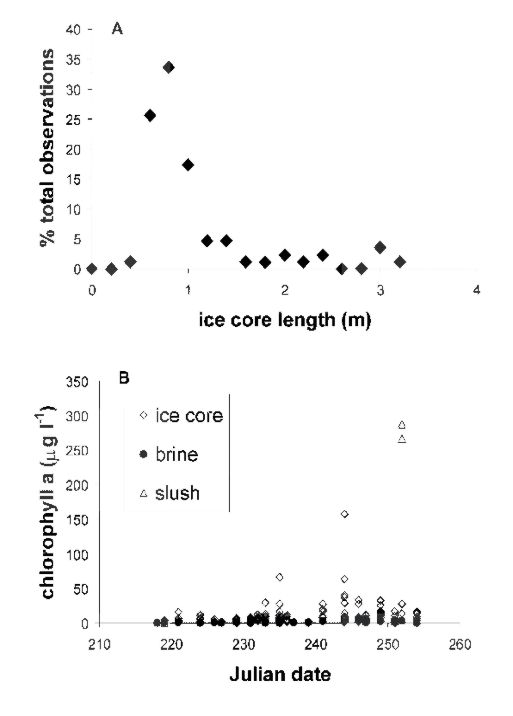 Figure 40. a) Frequency distribution of sea ice core lengths collected at 23 ice
stations on, or in the immediate vicinity of, the SO GLOBEC IV survey grid. b)
Chlorophyll
a concentrations in sea ice (ice core, brine, and slush) habitats sampled
during the SO GLOBEC IV survey cruise.
Figure 40. a) Frequency distribution of sea ice core lengths collected at 23 ice
stations on, or in the immediate vicinity of, the SO GLOBEC IV survey grid. b)
Chlorophyll
a concentrations in sea ice (ice core, brine, and slush) habitats sampled
during the SO GLOBEC IV survey cruise.
Science Party (Name, Institution )
Zooplankton and Krill Survey (BIOMAPER-II, 1-m MOCNESS, ROV) [BG247]
Wiebe, Peter Woods Hole Oceanographic Institution
Lawson, Gareth Woods Hole Oceanographic Institution
Thompson, Gustavo Universidad de Buenos Aires, Argentina
Alatalo, Philip Woods Hole Oceanographic Institution
Allison, Dicky Woods Hole Oceanographic Institution
Gallager, Scott Woods Hole Oceanographic Institution
Scott, Alec UK
Krill Distribution, Physiology, and Predation [BG236]
Daly, Kendra University of South Florida
Scolardi, Kerri University of South Florida
Yam, Emily University of Virginia
Zimmerman, Jason University of South Florida
ADCP/OPC/MOCNESS Studies [BG248]
Dorland, Ryan University of Massachusetts, Boston
Krill Physiology and Fish Ecology [BG245]
Torres, Jose University of South Florida
Bailey, Thomas University of South Florida
Donnelly Joe University of South Florida
Parker, Melanie University of South Florida
CTD/XBT/ADCP [OG240]
Hofmann, Eileen Old Dominion University
Salihoglu, Baris Old Dominion University
Beardsley, Bob Woods Hole Oceanographic Institution
Beardsley, Sue Woods Hole Oceanographic Institution
MacKay, Chris RGL Consulting, LTD Canada
Nutrients [OG266]
Serebrennikova, Yulia University of South Florida
Bell, Steve University of South Florida
Productivity Measurements [BG246]
Sines, Karie Scripps Institution of Oceanography
Stewart, Frank Scripps Institution of Oceanography
Seabird Survey/Ecology [BG-243]
Ribic, Chris University of Wisconsin
Chapman, Erik University of Wisconsin
Whale Survey/Active Counting
Viddi, Francisco Instituto Nacional Antartica de Chile
Distribution, Activity, and Dynamics of Sea Ice Microbiota [BG235]
Boc, Jenny University of Nevada
Raytheon Technical Support
Shepherd, Chris Marine Project Coordinator
Alesandrini, Stian Marine Technician
Ford, Nancy Marine Technician
Johnson, Jamee Marine Technician
Huckins, Paul Information Technology
Jackson, Patricia Information Technology
Gavahan, Kathleen Information Technology
Johnson, Todd Electronics Technician
Stuart, Fred Electronics Technician
Dizick, Sarah Marine Science Technician
Ship’s Officers and Crew
Borkowski, Joe Master
Watson, Mike Chief Mate
Repin, Vladimir Ice Pilot
Jarkiewicz, Paul 2nd Mate
Pagtalunan, Rachelle 3rd Mate
Munroe, Dave Chief Engineer
Pierce, Johnny 1st Engineer
Forbes, Edward 2nd Engineer
Welte, Frank 3rd Engineer
Zipperer, Bryan 3rd Engineer
Pagdanganan, Rogelio Oiler
Ambrocio, Ruel Oiler
Dela Cruz, Fredor Oiler
Alvezo, Enrique Oiler
Garde, Lauro A.B.
Tamayo, Ric A.B.
Aaron, Bienvenido A.B.
Villanueva, Sam A.B.
Carpio, Ronnie A.B.
Sandoval, Lorenzo A.B.
Stelly, Ernest A.B.
Silverio, Nestor O.S
Monje M., Alejandra A.B.
Arancibia, Claudia Duque O.S