WHOI Silhouette DIGITIZER
Version 1.0
Users Guide
by
William S. Little and Nancy J. Copley
Woods Hole Oceanographic Institution
WHOI Technical Report WHOI-2003-05


Acknowledgements
WHOI Silhouette DIGITIZER was developed at Woods Hole Oceanographic Institution as part of the GLOBEC (GLOBal ocean ECosystems dynamics) data management program.
DIGITIZER was devised by WHOI marine biologist and Senior Scientist Peter H. Wiebe as a modern and efficient method of counting and measuring marine organisms.Ā We the authors are greatly indebted to Dr. Wiebe, not only for his perception and creativity in suggesting this new digital approach to marine sampling, but also for his guidance, his encouragement, and especially his patience, during the long debugging period.ĀĀ Thanks Peter!
We would like to thank Research Assistant III Mari Butler and Information Systems Specialist Roger Goldsmith for their help in designing and testing portions of this software.
And we are particularly appreciative of the efforts of the many individuals who served as digitizing guinea pigs, and who therefore suffered the agonies associated with trying to do useful work with an endless series of software pre-releases.
WHOI Silhouette
DIGITIZER software and documentation were funded as part of
The National Science Foundation
GLOBEC program
grants OCE-9806381, OCE-9940880, and OCE-0095069.
* U.S.GLOBEC:ĀĀ Program Services and Data Management for Phase Three of the Northwest Atlantic Georges Bank Program, and follow-on.
MATLAB® is a product of The MathWorks, Inc.
WHOI Silhouette DIGITIZER
Version 1.0
Users Guide
*******************************************
TABLE OF CONTENTS
1.2ĀĀĀĀĀĀ MEASURING
MODES AND SAMPLE IDENTIFICATION
1.3ĀĀĀĀĀĀ REFERENCE
GRID, ZOOM, PAN, CALIBRATION, RANDOM CELLS
1.5ĀĀĀĀĀĀ SPECIES
SELECTION BUTTONS
1.7ĀĀĀĀĀĀ SAMPLE
LENGTH LIMITS
1.13ĀĀĀĀ SPREADSHEET-READABLE
TEXT OUTPUT FILES
1.14ĀĀĀĀ SPECIAL
SPECIES CODE AND SYMBOL
2.1.1Ā
initialization controls
2.1.2Ā
cell selection, zoom, and pan controls
2.1.3Ā
digitizing mode controls
2.1.4Ā
sample editing controls
2.3ĀĀĀĀĀĀ EDIT
SPECIES PARAMETERS WINDOW
2.3.1Ā
species color buttons 1 to 110
2.3.2Ā
changing the species color
2.3.3Ā
changing the species allowable length limits
2.3.4Ā
adding a species button to the Main Window
2.3.5Ā
verifying the color, allowed length, or main window visibility changes
2.3.6Ā
saving the color, allowed length, or main window visibility changes
2.3.7Ā
species color buttons Ā111-119
2.3.8Ā
species color button 120
2.4ĀĀĀĀĀĀ EDIT
COLORMAP WINDOW
2.5ĀĀĀĀĀĀ RANDOM
CELL GENERATOR WINDOW
2.6ĀĀĀĀĀĀ EDIT
PLATE PARAMETERS WINDOW
2.6.1Ā
setting parameters that are common to all species
2.6.2Ā
setting parameters that are specific to each species
2.6.3Ā
updating the test histogram
2.6.4Ā
setting parameters that affect the plotted and printed length histograms
2.6.5Ā
making a histogram plot
2.6.6Ā
writing a histogram file
3.1.1Ā
Select the input and output files
3.1.2Ā
Add your own measurements
3.1.4Ā
Save you results and quit DIGITIZER
3.2.1Ā
Initialize the calibration parameters and image reference grid:
3.2.2Ā
Edit the colormap of the image to improve its contrast.
3.2.3Ā
Change the allowable length limits for a species
3.2.4Ā
Make some measurements using theĀ
2-pointĀ mode
3.2.5Ā
Add a species button to the main menu and change its properties
3.2.6Ā
Measure a curved specimen using theĀ
ōn-pointöĀ mode
3.2.7ĀĀ
Save your results and quit DIGITIZER
3.3.1Ā
Remove measurements using select by cursor
3.3.2Ā
Change the species code of a measurement using select by number
3.3.3Ā
Delete multiple measurements at once using select by region
3.3.4Ā
Delete specimens of a single species using select by region
3.3.5Ā
Change species codes for several specimens at once using select by
region
3.3.7Ā
Save your results and quit DIGITIZER
3.4.1Ā
Create an output statistics file
3.4.2Ā
Create output length and weight files
3.4.3Ā
Create a histogram plot of the measured sample lengths
3.4.4Ā
Create a histogram file of the measured sample lengths
3.4.5Ā
Create a histogram file of the counts of the measured samples
3.4.6Ā
Create a histogram file of the weights of the measured samples
3.4.7Ā
Save you results and quit DIGITIZER
3.5.2Ā
Making a new species file
3.5.3Ā
Making a new weights file
3.5.4Ā
Changing the weights file during a session
3.5.5Ā
Recalculating the weights of existing measurements.
3.5.6Ā
Save you results and quit DIGITIZER
4ĀĀĀĀĀ SYSTEM REQUIREMENTS AND
RESTRICTIONS
6ĀĀĀĀĀ SOFTWARE ON CD-ROM AND THE WEB
Appendix 1ĀĀĀĀ Standard Lengths Used in
DIGITIZER Program
Appendix 2ĀĀĀĀ Length to Wet Weight
Biomass Conversion Formulas.
1ĀĀĀĀĀĀĀĀĀ PROGRAM DESCRIPTION
1.1ĀĀĀĀĀĀ OVERVIEW
WHOI Silhouette DIGITIZER is a MATLAB-based computer
program for measuring the lengths of marine organisms in the macrozooplankton
size range.
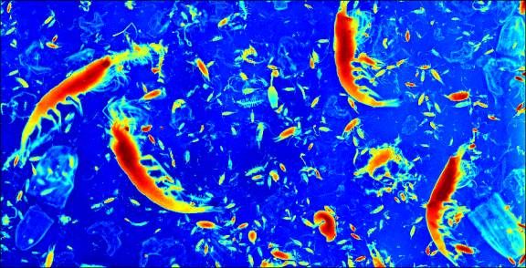
DIGITIZER begins by displaying a scanned photographic image
of a seawater slurry containing large numbers of marine organisms, upon which
is superimposed a reference grid.Ā
DIGITIZER then allows you to measure the organisms' lengths using the
cursor on the computer screen.Ā
DIGITIZER automatically calculates each organismÆs biomass and generates
spreadsheet compatible output listings of basic statistics derived from the
data.ĀĀ DIGITIZER also produces text
files of lengths, weights, and size-frequency histograms.
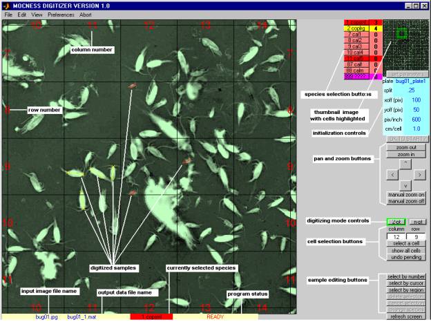
The DIGITIZER Main Window shown here contains a portion of a typical scanned image and several digitized samples, along with various control buttons, information boxes and edit boxes. Detailed descriptions of these elements are presented in subsequent sections of this document.
When you measure a sample in the Main Window, you perform three basic steps:
(1) you select an area of the image using the cell selection, pan, and zoom controls;
(2) you select a species to digitize using the appropriate colored species selection button;
(3) you click on one end of an organism on the image, and then click on the other end of the organism.
You can also measure the length of a curved organism by first clicking on the "n-pt" button to change the program to multi-point ("n-point") mode.Ā Once the species is selected, you click on one end of the sample, hold the mouse button down while tracing the cursor along the organism, and release the mouse button at the other end of the organism.
When you make a measurement, in the MATLAB command window will appear the number of the measurement, the species code, the organism's length, the organism's weight, and the grid cell coordinates.Ā This allows you to check your measurements as you go along.
Colored selection buttons representing various species may be added to (or removed from) the Main Window by selecting "edit species buttons, lengths" from the Edit Menu.Ā This creates an Edit Species Parameters Window that can be used to change the color and availability (visibility) of each species button.Ā You can also use this window to change the maximum and minimum allowed sample lengths for each species, so that digitized samples that exceed these limits are automatically rejected.
Certain properties of the image that appears in the Main Window may be altered by selecting the "edit colormap" from the Edit Menu.Ā This creates an Edit Colormap Window whose controls can be used to change the overall image color (tint) and the image "exposure curve" in order to make the organisms in the image more distinct.
DIGITIZER provides several options under the File Menu of the Main Window for writing the raw data and derived statistics to disk files.
Section 1 of this Users Guide gives an overview of the important features of DIGITIZER.
Section 2 is a reference section that explains DIGITIZER's windows and Graphical User Interface (GUI) controls.
Section 3 contains some simple tutorials that illustrate many of DIGITIZER's features.
Section 4 discusses the system requirements for running DIGITIZER.
Section 5 lists some known problems that exist in DIGITIZER Version 1.0.
Appendix 1 shows a variety of zooplankton types with
guides for making standard length measurements.
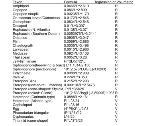
Appendix 2 contains a list of formulas used for length
to wet weight biomass conversions.
Software on a CD-ROM is included at the back of this technical report that allows you to install DIGITIZER version 1.0 on Windows 98 or Windows 2000 ( and Windows XP).Ā The folders contain æp filesÆ for Matlab versions 6.1 and 6.5.
Before proceeding, please read Section 4.Ā It describes some known bugs and operational problems involving the way DIGITIZER interacts with the Windows Operating System.Ā In some cases these may make DIGITIZER awkward to use, or even unusable, on your computer!Ā Along with The MathWorks, Inc., the provider of MATLAB, we are working to correct these deficiencies.
If you are curious about how to use DIGITIZER, you may at this point skip directly to the Tutorials in Section 3
1.2ĀĀĀĀĀĀ MEASURING MODES AND SAMPLE IDENTIFICATION
DIGITIZER provides two measuring
modes, the 2-point mode where only the organism's two end points are used to
determine its length, and the n-point mode where the organism's length is
measured along a curve traced by the cursor.
Each measured organism is
identified by a species code which is selected by clicking on the appropriate
species button, either at the beginning of a series of measurements or after
making each measurement.
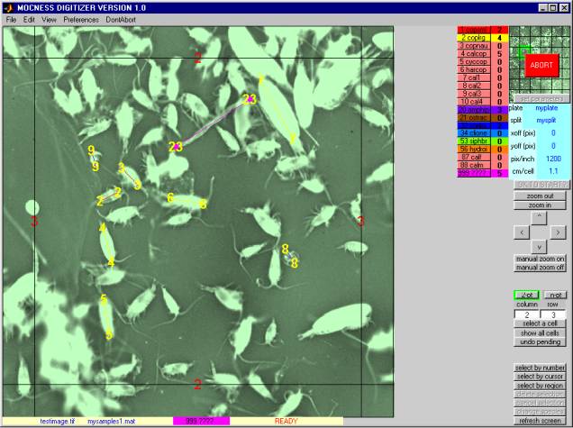
As measurements are made, the
program draws colored lines on the image to show which organisms have been
measured.Ā It numbers the measurements
for easy identification and subsequent editing.Ā These numbers can be turned on or off and their size changed.
1.3ĀĀĀĀĀĀ REFERENCE GRID, ZOOM, PAN, CALIBRATION, RANDOM CELLS
DIGITIZER superimposes a square
reference grid on the displayed image and allows the user to magnify portions
of the image by "zooming" in on individual grid cells or groups of
cells, or move about the image by "panning" horizontally or
vertically.
Prior to making measurements,
the user must enter the resolution of the image, typically the resolution
setting of the scanner that was used to create the image.Ā The user may optionally position the
reference grid by moving it a number of pixels vertically and/or horizontally.
In instances where there are too
many organisms of a given type to justify measuring every individual organism,
DIGITIZER provides a means of generating a list of randomly located cells.Ā Measurements may then be made only in the
cells on the random cell list, thereby providing a means of systematically
subsampling the overall image.
1.4ĀĀĀĀĀĀ IMAGE FILES
DIGITIZER reads image files that
are compatible with the MATLAB "imread" function, for example,
".tif" or ".jpg" files.Ā
It displays images using a 256-level single-tint "colormap"
whose exposure curve and hue may be altered for easier viewing or more accurate
measuring.
The input image file is generally
created using a digital scanner and the accompanying vendor supplied scanner
software.Ā A typical image of a scanned
6" X 8" black and white photographic negative would contain 7200 X
9600 pixelsĀ (picture elements) when
scanned at 1200 X 1200 pixels per inch. At 256 intensity levels per pixel (8
bits per pixel) this would result in a total image size of 69.12 Mbytes.Ā An 8" X 10" film requires about
110 Mbytes.
1.5ĀĀĀĀĀĀ SPECIES SELECTION BUTTONS
In general, a large number of
species selection buttons are displayed on the screen, together with other
function buttons, program status information, and the actual image.Ā In order to reduce screen clutter, the user
may edit the species button list so that the screen displays only those buttons
corresponding to the organisms which are most likely to be encountered during a
particular measuring session.Ā
Measurement size limits for each species button can also be
established.Ā Samples with measured
lengths outside of these limits are automatically rejected (see below).
1.6ĀĀĀĀĀĀ DATA EDITING
Samples that have been measured
incorrectly can be deleted from the screen and from the output data files.Ā The species codes of individual measurements
or nearby groups of measurements can also be altered to correct for previous
species selection errors.Ā The user can
select the sample to be altered either by using the cursor to pick out the
desired sample on the image, by specifying the sample number, or by selecting a
region using a "rubber band" box.Ā
When a measurement lies partially within the rubber band box, the
criteria for determining whether or not it is ōselectedö may be specified as
ōone end in the boxö, or ōboth ends in the boxö, as set in the preferencesnces
menu.
1.7ĀĀĀĀĀĀ SAMPLE LENGTH LIMITS
DIGITIZER checks measurements for
legal lengths.Ā If the measured length
of a particular sample is out of the
range of acceptable values for the selected species, the sample is rejected,
the computer beeps or clicks, and the corresponding data are removed from the
screen and from the output data files.
The maximum and minimum acceptable
lengths for each species may be set by the user, and may be overridden when
necessary by changing the limits settings.
1.8ĀĀĀĀĀĀ WEIGHT CALCULATIONS
In cases where the appropriate
formula is supplied to the program, DIGITIZER uses each organism's length to
automatically calculate its weight (biomass).Ā
The formulas are provided in an editable ASCII file, default.wgt, in the
form of equations that are MATLAB compatible.Ā
Most of the formulas provided in default.wgt were derived by Davis and
Wiebe (1985)* for zooplankton forms from warm North Atlantic waters.Ā Care should be taken in interpreting wet
weight data from this program when applied to your samples.
*ĀĀĀĀĀĀĀĀĀĀĀĀĀ Wiebe, P. H. and C. S. Davis. 1985. ōMacrozooplankton biomass in a warm-core Gulf Stream ring: Time series changes in size structure, taxonomic composition, and vertical distribution.ö J. Geophys. Res. 90(C5):8871-8884.
1.9ĀĀĀĀĀĀ DATA LOGGING
As measurements are made, the
image coordinates and the calculated lengths and weights are listed in the
MATLAB command window, which may be scrolled backward if necessary in order to
examine previous data.Ā Measurements
that result in illegal lengths are marked as either too long or too short.
1.10ĀĀĀĀ INPUT PARAMETERS
DIGITIZER allows the user to establish the default values of
several program parameters, such as species button colors, species length
limits, weight formulas, grid size, and image resolution.Ā Some input parameters can be interactively
changed during a measuring session using a species button editing window.
1.11ĀĀĀĀ BINARY OUTPUT FILES
DIGITIZER stores the measured data
in two ways.Ā All measured coordinates
are initially entered into a collection of tables in memory in the MATLAB main
workspace.Ā These tables are
periodically saved to a MATLAB binary ".mat" file,.Ā This occurs after every twentieth sample,
whenever a previously measurement is altered or deleted, and whenever the user
requests it by explicitly selecting one of several file /save options.Ā These memory tables and disk files
constitute a complete record of all measurements made on a particular image.
Whenever a new session of DIGITIZER begins, the program automatically makes a backup copy of theĀ .mat file, giving it the same filename as theĀ .mat file but with the file extensionĀ ".mbk".Ā Then, if the operating system or the program crashes or otherwise exhibits erratic behavior, you can always quit or abort DIGITIZER and discard your corruptedĀ .mat file.Ā You can later rename theĀ .mbk file as aĀ .mat file and use it to resume measuring with DIGITIZER.Ā You will lose the measurements from the most recent session, but you will not lose measurements that were made during previous sessions using this image.
1.12ĀĀĀĀ TEXT OUTPUT FILES
When the data in the memory tables
are written to a binary file, they are also written to an ASCII text file which
has the file extension ō.datö.Ā Unlike
the .mat file, this ASCII file is human-readable, and may be listed on a
printer or imported into a spreadsheet program for further analysis.Ā For each measurement, the file contains the
species code, cell location, calculated length and weight, and information
identifying the particular image.
The internal data tables and the
binary output file contain all digitized information, including data pertaining
to samples whose lengths were found to be illegal, and data for samples which
were deleted from the screen using the programs editing features.Ā The text file, however, contains only
"good" samples; illegal length samples and deleted samples are not
recorded.
The binaryĀ .matĀ
file and the ASCII textĀ
.datĀ file are both completely
rewritten whenever existing measurements are deleted or species codes are
retroactively changed by the user.
1.13ĀĀĀĀ SPREADSHEET-READABLE TEXT OUTPUT FILES
The program allows the user to
write a number of text files that may be easily imported into the EXCEL
spreadsheet program.Ā Files may be
created that include the lengths of the samples, weights of the samples, some
basic sample statistics for the overall sample collection, and histogram data
of sample counts, sample weights, or sample lengths.
1.14ĀĀĀĀ SPECIAL SPECIES CODE AND SYMBOL
DIGITIZER provides a special
species code (999) and symbol (large magenta dot) that serves as a means of
marking an item of special interest on the image (something to be looked at
again later but not identified yet).Ā
The coordinate data associated with the special species code are
recorded in the internal data tables and the binary output file, but are
omitted from the text output file.
2ĀĀĀĀĀĀĀĀĀ WINDOWS AND MENUS
2.1ĀĀĀĀĀĀ MAIN WINDOW
The Main Window of DIGITIZER looks something like this.Ā Its control elements are described in the following sections.
2.1.1Ā initialization controls
set parametersĀĀĀĀĀĀĀĀĀĀĀĀĀ click
on this control to temporarily apply your settings so you can see what the
image looks like with its new calibration data and grid lines.
plateĀĀĀĀĀĀĀĀĀĀĀĀĀĀĀĀĀĀĀĀĀĀĀĀĀĀĀĀ enter the "plate name", that is, any ASCII name you wish to use for the samples you digitize from this image (for example, "myplate001" ).
(In this
Users Guide, the word "plate" is essentially synonymous with the word
"image", as in "photographic plate" or "photographic
image").
splitĀĀĀĀĀĀĀĀĀĀĀĀĀĀĀĀĀĀĀĀĀĀĀĀĀĀĀĀĀ enter
a "split factor", that is, any numeric fraction that represents the
portion of the overall sea water sample you used when creating the image for
this sessionĀ ( for example:Ā 1 , orĀ
1 / 4 , or 0.125 ).
pix/inchĀĀĀĀĀĀĀĀĀĀĀĀĀĀĀĀĀĀĀĀĀĀĀĀ enter
the number of "pixels per inch" of the originating image.Ā This is typically the resolution used by the
scanner in creating the image file (for example, 1200).Ā (A future version of the program may provide
for on-screen calibration using reference marks on the scanned image.)
cm/cellĀĀĀĀĀĀĀĀĀĀĀĀĀĀĀĀĀĀĀĀĀĀĀĀĀ enter
the cell (square) size in centimeters to determine the reference grid size (for
example, 2.0).Ā For historic reasons,
the default is 1.1.
xoff (pix)ĀĀĀĀĀĀĀĀĀĀĀĀĀĀĀĀĀĀĀĀĀ enter
an integer number of pixels to offset (shift) the reference grid to the left or
rightĀ ( for example, 50 ).
yoff (pix)ĀĀĀĀĀĀĀĀĀĀĀĀĀĀĀĀĀĀĀĀĀ enter
an integer number of pixels to offset (shift) the reference grid up or
downĀ ( for example, -100 ).
OK TO START?ĀĀĀĀĀĀĀĀ click
on this control to make the parameter settings permanent for all digitizing
sessions associated with this image.Ā A
message box will appear asking you to confirm your selection
2.1.2Ā cell selection, zoom, and pan controls
column,Ā rowĀĀĀĀĀĀĀĀĀĀĀĀĀĀĀ enter integer column and row
numbers (refer to the red reference numbers on the image)Ā and then click on "select a cell"
to zoom directly to an individual grid cell.
select a
cellĀĀĀĀĀĀĀĀĀĀĀĀĀĀĀĀĀĀ click on this to
zoom to a selected cell.
show all
cellsĀĀĀĀĀĀĀĀĀĀĀĀĀĀĀ click on this to
restore the full size image.
zoom out, zoom inĀĀĀĀĀĀĀ when
you have selected an individual cell, click on these controls to expand or
contract the image area to include more than one cell.
<ĀĀ >ĀĀ
^ĀĀ vĀĀ
when you
have selected an individual cell (or small collection of cells),Ā you can click on these controls to
"pan" the image one cell to the left, one cell to the right, one cell
up, or one cell down, respectively.
manual zoom onĀĀĀĀĀĀĀĀĀĀĀ click
on this control to temporarily change the behavior of the cursor so that it can
be used to zoom to an arbitrary area of the image.Ā After clicking on this control, you can use the cursor to select
a rectangular area by pressing the mouse button at one corner of the desired
area and dragging it to the diagonally opposite corner of the desired
area.Ā A new enlarged image area will
appear.
Subsequent clicks of the left mouse button will cause the image to zoom in, while clicking the right mouse button will zoom out.Ā The new image will be re-centered at the position of the cursor.Ā Double clicking the left mouse button will restore the image to its original size just prior to your first zoom.
You MUST
click on "man zoom off" (see below) before proceeding with
digitizing, in order to return the cursor behavior to normal.Ā If you don't, you will inadvertently
continue zooming instead of measuring!
manual zoom offĀĀĀĀĀĀĀĀĀĀ click
on this control to return the cursor behavior to normal so that you can
continue digitizing.Ā (If you forget to
do this, try using "undo pending" and/or the sample editing controls
(see below) to reset the program status to READY and eliminate accidentally
digitized data.)
(TheĀĀ "manual zoom on/off"ĀĀ buttons simply execute the MATLAB
functionsĀ "zoom
on"/"zoom off"Ā
functions, thus enabling/disabling all of the standard MATLAB
cursor-controlled zoom features.)
2.1.3Ā digitizing mode controls
2-ptĀĀĀĀĀĀĀĀĀĀĀĀĀĀĀĀĀĀĀĀĀĀĀĀĀĀĀĀĀ click
here when you wish to digitize subsequent samples using only two points, that
is, to measure sample lengths along a straight lines.
n-ptĀĀĀĀĀĀĀĀĀĀĀĀĀĀĀĀĀĀĀĀĀĀĀĀĀĀĀĀĀ click
here if you want to digitize a sample using multiple points along the curve
which you trace with the cursor from one end of an organism to the other.Ā This control works in conjunction with the
"n-point digitizing mode" menu item under Preferences on the Main
Window menu bar, as follows:
If the
"n-point digitizing mode" option is set to "n-pt
persistent", the program will not return to 2-pt mode until you click the
"2-pt" control.
If
theĀ "n-point digitizing mode"
option is set to "n-pt one-shot", the program mode will automatically
return to 2-point mode after each measurement.
2.1.4Ā sample editing controls
select by numberĀĀĀĀĀĀĀĀĀĀ click
here to select a sample for editing by referring to it by its sample number.
select by cursorĀĀĀĀĀĀĀĀĀĀĀ click
here to select a sample for editing by clicking on the sample with the cursor.
select by regionĀĀĀĀĀĀĀĀĀĀĀĀ click
here to select all of the samples in a rectangular region for editing, using to
cursor to specify the desired area.
delete selectionĀĀĀĀĀĀĀĀĀĀĀĀ click
here to actually eliminate the sample(s) you have selected for editing.
cancel selectionĀĀĀĀĀĀĀĀĀĀĀĀ click
here if you change your mind and decide NOT to delete or alter the samples you
have selected for editing.
change speciesĀĀĀĀĀĀĀĀĀĀĀĀĀ click
here to change the species of the sample(s) you have selected for editing.
The
resulting message box will ask you if you want to change the species code of
ONE species or ALL of the length measurements in the selected region.Ā (You can also CANCEL the overall selection.)
If the
answer is ALL, next click on the species button of the new species you wish to
assign to all the selected samples.
If the
answer is ONE, you must first click on a species button to indicate which
species within the selected region you wish to change.Ā You must next click on the species button of
the new species you wish to assign to the selected samples.
A
message box will appear asking you to confirm your change(s), after which the
program will re-calculate sample weights, update the measurement lines on the
image, and update the output .mat and .dat files.
Samples
will be deleted if they no longer satisfy the length restrictions associated
with the new species assignment.Ā A
mistake here can cause you to lose previously measured lengths.
2.1.5Ā species buttons
click on
one of these colored controls to select the species you wish to assign to
subsequent digitized samples
2.1.6Ā species counts
these
colored boxes, which are adjacent to each species button, indicate the total
number of successfully digitized samples of each species.Ā The counts do not include samples that have
been manually deleted, or those automatically rejected because they are of
illegal length.
2.1.7Ā information box
displays
the names of the input image file and the output .mat data file.Ā It is located at the bottom of the window.
2.1.8Ā selected species box
displays
the species name, species code number, and color of the currently selected
species.Ā It is located at the bottom of
the window, next to the information box.
2.1.9Ā status box
displays
the status of the program.Ā A status of
READY indicates that the program is able to accept new digitized input, that
is, the cursor is enabled to record image coordinates either for 2-point or
n-point mode.Ā Here is a complete list
of status messages, most of which are self-explanatory.
BACKING UPTO .mbk FILE
CREATING
SPECIES BUTTONS
DEL, CANCEL, OR CHANGE SPEC
ENTER IMAGE PARAMETERS
ENTER A SAMPLE NUMBER
MAKING SPEC/LEN EDITOR
OPENING OUTPUT FILES
PRESS A SPECIES BUTTON
READING IMAGE FILE
READING SAMPLE 150 of 500
READY
REPLOTTING SAMPLES
SELECT SAMPLE BY CURSOR
SELECTING SPECIES BUTTONS
WAITING FOR POINT 2
WAITING FOR SPECIES CODE
WAITING
TO SELECT REGION
2.1.10Ā refresh screen
Occasionally
the program (or the operating system) gets confused and fails to update the
display with the most recent graphics information.Ā If you think this has happened, try using this button to execute
a MATLAB refresh command.Ā This will
often fix the problem.
2.1.11Ā undo pending
If you
change your mind part way through a sequence of point and click operations and
wish to return to READY status, click on this button.
2.1.12Ā ABORT
This is
the "kill" button!ĀĀ When the
program hangs or some other unusual event occurs, use this button to stop the
program without writing anything more to any files.Ā The button essentially wipes out all windows and exits MATLAB
immediately.Ā It should be used only in
an emergency.Ā After clicking on Abort, a
red button will appear in the upper right corner of the window.Ā Click on the red button to actually abort
the program.Ā Or, if you change your
mind, click on "DontAbort" on the menu bar to make the red button
disappear.
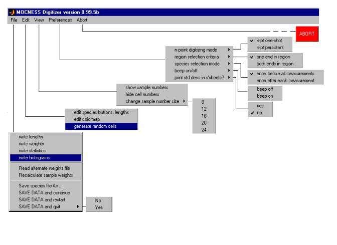
2.2ĀĀĀĀĀĀ MAIN WINDOW MENUS
Here is a diagram showing the hierarchy of DIGITIZER Main Window pull-down menu options, each of which is described in the subsections that follow.
2.2.1Ā File
writeĀ lengthsĀĀĀĀĀĀĀĀĀĀĀĀĀĀĀĀĀĀĀĀĀĀĀĀĀĀĀĀĀĀĀĀĀĀĀĀĀĀĀ writes a
text file containing all the measured length data.
writeĀ weightsĀĀĀĀĀĀĀĀĀĀĀĀĀĀĀĀĀĀĀĀĀĀĀĀĀĀĀĀĀĀĀĀĀĀĀĀĀĀ writes a text file containing all of the derived sample weights which have been calculated from measured lengths, using the weight formulas in the currently active weightĀ file (default.wgt or your own alternativeĀ .wgtĀ file).
writeĀ statisticsĀĀĀĀĀĀĀĀĀĀĀĀĀĀĀĀĀĀĀĀĀĀĀĀĀĀĀĀĀĀĀĀĀĀĀĀĀ writes a
text file containing basic statistics derived from the lengths of the measured
samples.Ā This includes the minimum,
maximum, and mean, as well as the sample count for each species.Ā It also (optionally) includes the sample
standard deviation and the population standard deviation for each species.
writeĀ histogramsĀĀĀĀĀĀĀĀĀĀĀĀĀĀĀĀĀĀĀĀĀĀĀĀĀĀĀĀĀĀĀĀĀĀ brings up the
Edit Plate Parameters Window.
This
window allows you to enter all of the experimental parameters associated with
the image that DIGITIZER needs in order to calculate abundance and biomass.
It
allows you to generate histogram files of your data, separated into bins
according to length, weight, or sample count.
In the
case of sample lengths, the window provides controls for specifying the
particular method of assigning length bins, and for subsequently plotting
histograms (bar plots).
(Note:ĀĀĀ The length, weight, statistics, and
histogram text files may be easily imported into Microsoft EXCEL spreadsheet,
using the following sequence of Version 2000 EXCEL menu and option choices:Ā File/Open, Delimited, Space Delimiters,
Finish.)
Read alternate weights fileĀĀĀĀĀĀĀĀĀĀĀĀĀĀĀĀĀĀĀĀ provides a means of changing the file from which are imported the formulas for calculating weights as functions of lengths for various species.
Recalculate sample weightsĀĀĀĀĀĀĀĀĀĀĀĀĀĀĀĀĀĀ allows you to actually use the formulas in the alternate weights file (read in above) to recalculate the weights of all the previously measured samples A WARNING message is issue because all future statistics will be based on the new weight formulas, thus making previous results invalid.
Save species file As... ĀĀĀĀĀĀĀĀĀĀĀĀĀĀĀĀĀĀĀĀĀĀĀĀ writes
a new species parameter file that may be used for future DIGITIZER sessions
instead of the default species parameter file "default.men".Ā Species parameter files have the file
extension .men.Ā They are text files
which may be (carefully) edited with a text editor to alter species colors,
length limits, and/or the visibility of species buttons on the main menu.
SAVE DATA and continueĀĀĀĀĀĀĀĀĀĀĀĀĀĀĀĀĀĀ saves
your latest measurements in the current outputĀ
.mat andĀ .dat files.
You
should execute this option whenever you what to insure that your latest
measurements are permanently recorded.
Even if
you don't do this, the program automatically does it after every 20 new
samples, as well as whenever existing measured samples are deleted or their
species codes changed.
SAVE DATA and restartĀĀĀĀĀĀĀĀĀĀĀĀĀĀĀĀĀĀĀĀĀ saves
your latest measurements in the current outputĀ
.mat andĀ .dat files, resets all
of the programÆs internal variables and data tables, and allows you to begin a
new digitizing session.
SAVE DATA and quitĀĀĀĀĀĀĀĀĀĀĀĀĀĀĀĀĀĀĀĀĀĀĀĀĀ saves
your latest measurements in the current output .mat and .dat files, quits
DIGITIZER, and exits MATLAB.
Selecting
this option brings up another submenu which requires you to confirm that you
wish to quit (Yes), or else change your mind and continue digitizing (No).
2.2.2Ā Edit
edit species buttons, lengthsĀĀĀĀĀĀĀĀĀĀĀĀĀĀĀĀĀ opens the Edit Species Parameters Window (described
in Section 2.3)
edit colormapĀĀĀĀĀĀĀĀĀĀĀĀĀĀĀĀĀĀĀĀĀĀĀĀĀĀĀĀĀĀĀĀĀĀĀĀĀĀ opens
the Edit Colormap Window (described in Section 2.4)ĀĀĀ
generate random cellsĀĀĀĀĀĀĀĀĀĀĀĀĀĀĀĀĀĀĀĀĀĀĀĀĀĀ opens
the Random Cell Generator Window (described in Section 2.5)
2.2.3Ā View
show (hide) sample numbersĀĀĀĀĀĀĀĀĀĀĀĀĀĀĀĀ optionally
displays yellow sample numbers at both ends of each digitized sample on the
image.Ā The size of the text font used
for sample numbers may be changed using the "change sample number
size" submenu option (below).
hide (show) cell numbersĀĀĀĀĀĀĀĀĀĀĀĀĀĀĀĀĀĀĀĀĀĀ optionally
displays red cell numbers near the edges of the displayed image.
change sample number sizeĀĀĀĀĀĀĀĀĀĀĀĀĀĀĀĀĀĀ allows
you to change the font size of the yellow sample numbers.Ā The choices are theĀ 8, 12, 16, 20, and 24 point fonts.
2.2.4Ā Preferences
n-point digitizing modeĀĀĀĀĀĀĀĀĀĀĀĀĀĀĀĀĀĀĀĀĀĀĀĀĀ This
option works only when the program is in n-point mode, as determined by the
"n-pt" control button on the Main Window. The two choices are:
n-pt one-shotĀĀĀĀĀĀĀĀĀĀĀĀĀĀĀĀĀĀĀĀĀĀĀĀĀĀĀ with
this selection, the program will revert automatically to 2-pt mode after a
single n-point measurement has been made.
n-pt persistentĀĀĀĀĀĀĀĀĀĀĀĀĀĀĀĀĀĀĀĀĀĀĀĀĀĀ with
this selection, the program will remain in n-pt mode as long as the Main Window
"n-pt" mode button has been selectedĀ
(i.e., highlighted in green).
The
program will return to 2-pt mode when either the Main Window 2-pt mode button
is clicked, or the above "2-pt one-shot" option is selected and one
more sample is digitized.
region selection criteriaĀĀĀĀĀĀĀĀĀĀĀĀĀĀĀĀĀĀĀĀĀĀĀĀĀ This
option affects the manner in which previously digitized samples are chosen for
editing (removal or a change in species code)Ā
when the "select by region" button is activated on the Main
Window.Ā The two options are:
one end in regionĀĀĀĀĀĀĀĀĀĀĀĀĀĀĀĀĀĀĀĀĀĀĀĀĀĀĀĀĀĀĀĀĀ if
either end of a sample lies within theĀ
red selection box, that sample will be included in the selection.
both ends in regionĀĀĀĀĀĀĀĀĀĀĀĀĀĀĀĀĀĀĀĀĀĀĀĀĀĀĀĀĀĀĀ the
sample will be included in the selection only if both its ends lie within the
red selection box.
(Note: The program
does NOT look at intermediate points, so the fact that a sample track passes
through the red selection box is not sufficient to include the sample in the
selection.)
species selection modeĀĀĀĀĀĀĀĀĀĀĀĀĀĀĀĀĀĀĀĀĀĀĀĀĀ This
option affects the functioning of the species selection buttons in the Main Window.Ā The two choices are:
enter before all measurementsĀĀĀĀĀĀĀĀĀĀĀĀĀĀ This option specifies that once you have chosen a
particular species using one of the species selection buttons on the Main
Window, that selection stays in effect until you choose another species.Ā This is the normal (default) option.
enter after each measurementĀĀĀĀĀĀĀĀĀĀĀĀĀĀĀ This option specifies that you MUST, after digitizing
each sample, immediately click on one of the species selection buttons on the
Main Window, before proceeding to digitize another sample.Ā This option is provided for situations where
the species of the sample to be digitized changes very frequently
print std devs in s'sheets?ĀĀĀĀĀĀĀĀĀĀĀĀĀĀĀĀĀĀĀĀĀ This
options enables or disables the printing of population standard deviations and
sample standard deviations in the histogram and statistics output files.Ā The choices are yes and no.Ā The default is yes.
beep on/offĀĀĀĀĀĀĀĀĀĀĀĀĀĀĀĀĀĀĀĀĀĀĀĀĀĀĀĀĀĀĀĀĀĀĀĀĀĀĀĀĀĀ This
option determines whether or not an audible beep occurs when attempting to
digitize samples of illegal length.Ā The
submenu choices are on, and off.
stops DIGITIZER and MATLAB without saving the latest digitizer data or parameter changes.Ā To actually complete the Abort process, you must click on the red "ABORT" button that appears in the upper right corner of the screen.Ā If you change your mind, click "DonÆt Abort" on the menu bar.
2.3ĀĀĀĀĀĀ EDIT SPECIES PARAMETERS WINDOW
When you select the "edit species buttons, lengths" of the Edit pull-down menu, DIGITIZER creates the Edit Species Parameters Window, which looks like this.Ā The subsections below describe the various control items, which may be used to change the color of the species buttons, alter the sample legal length limits associated with each species, and either show or hide individual species buttons in the Main Window.
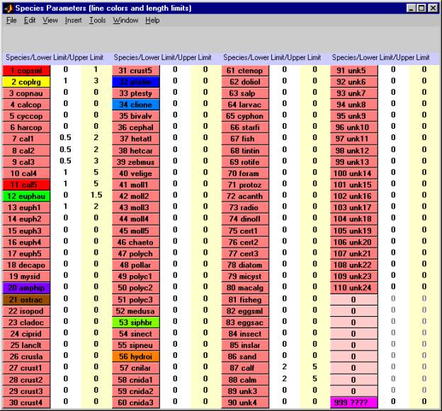
There are three kinds of species buttons in the Edit Species Parameters window:
buttons 1Ā to 110Ā (various colors)Ā are standard species selection buttons;
buttons 111 to 119Ā (pinkĀ andĀ unnumbered)Ā are for setting up groups of species for purposes of generating statistics for combinations ofĀ species
button 120Ā (magenta)Ā is the special species button (labeled "999 ????") for highlighting any object in the image with a "marker" dot.
2.3.1Ā species color buttons 1 to 110
Clicking on one of these buttons brings up another smaller sub-window which contains controls for changing (a) the color associated with this species, (b) the minimum and maximum allowable lengths for measurements of this species, and (c) whether or not this species button appears on the main menu.
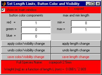
2.3.2Ā changing the species color
The color associated with a particular species is determined
by the settings of the three color components labeled red, green, and,
blue.Ā The color choice affects both the
color of the species button on the Main Window and the color of the lines drawn
on the image when you measure specimens of that species.Ā To change the color of a species, you change
the setting of each the three color components to a fraction betweenĀ 0.0Ā
andĀ 1.0.
Be sure to press "enter" on the keyboard to
successfully change each component.
The settings for several primary (bright) colors are listed below.
ĀĀĀĀĀĀĀĀĀĀĀ redĀĀĀĀĀĀĀĀĀĀĀĀĀĀĀĀĀĀ 1.0ĀĀĀĀĀĀ 0.0ĀĀĀĀĀĀ 0.0
ĀĀĀĀĀĀĀĀĀĀĀ yellowĀĀĀĀĀĀĀĀĀĀĀĀĀ 1.0ĀĀĀĀĀĀ 1.0ĀĀĀĀĀĀ 0.0ĀĀĀĀĀĀ (because red and green make yellow*)
ĀĀĀĀĀĀĀĀĀĀĀ greenĀĀĀĀĀĀĀĀĀĀĀĀĀĀĀ 0.0ĀĀĀĀĀĀ 1.0ĀĀĀĀĀĀ 0.0
ĀĀĀĀĀĀĀĀĀĀĀ cyanĀĀĀĀĀĀĀĀĀĀĀĀĀĀĀĀ 0.0ĀĀĀĀĀĀ 1.0ĀĀĀĀĀĀ 1.0ĀĀĀĀĀĀ (because green and blue make cyan*)
ĀĀĀĀĀĀĀĀĀĀĀ blueĀĀĀĀĀĀĀĀĀĀĀĀĀĀĀĀĀ 0.0ĀĀĀĀĀĀ 0.0ĀĀĀĀĀĀ 1.0
ĀĀĀĀĀĀĀĀĀĀĀ magentaĀĀĀĀĀĀĀĀĀĀĀ 10.ĀĀĀĀĀĀ 0.0ĀĀĀĀĀĀ 1.0ĀĀĀĀĀĀ (because
blue and red make magenta*)
ĀĀĀĀĀĀĀĀĀĀĀ whiteĀĀĀĀĀĀĀĀĀĀĀĀĀĀĀ 1.0ĀĀĀĀĀĀ 1.0ĀĀĀĀĀĀ 1.0
ĀĀĀĀĀĀĀĀĀĀĀ blackĀĀĀĀĀĀĀĀĀĀĀĀĀĀĀ 0.0ĀĀĀĀĀĀ 0.0ĀĀĀĀĀĀ 0.0
(*Note:Ā These rules apply to "additive" color systems such as those used on display monitors;Ā you should consult a textbook on color theory for an explanation of how this differs from the "subtractive" color systems used by printers.)
You can experiment with creating other colors, by choosing intermediate values for one or more of the primary color components in the above table.
For example, here's how to turn a bright color into a pastel.Ā Just add a few tenths to the smallest color component(s) such as the zero(s).Ā Thus, red (1.0ĀĀ 0.0ĀĀ 0.0) becomes pink (1.0Ā 0.75Ā 0.75),Ā orĀ yellow (1Ā 1Ā 0)Ā becomes pale yellowĀ (1.0ĀĀ 1.0ĀĀ 0.5).
You can darken a color, for example, you can convert orange (which is full red plus half green)Ā (1.0ĀĀ 0.5ĀĀ 0.0) into brownĀ (which is dark orange)Ā (0.7ĀĀĀ 0.4ĀĀ 0.0) by decreasing the larger of the color component(s) by a few tenths.
2.3.3Ā changing the species allowable length limits
Change the maximum and/or a minimum allowable species length (in millimeters) in the max and min edit boxes.Ā Any subsequent measurement of this species will be rejected if its length is found to lie outside of these new limits.
2.3.4Ā adding a species button to the Main Window
To add a button for this species to the Main Window, check the "show on main window" box in the upper left corner of the Set Length Limits ģ window.
2.3.5Ā verifying the color, allowed length, or main window visibility changes
To have either a new color/visibility combination or new length limits take effect in the Edit Species Parameters Window, click on the appropriate "apply color/visibility change" or "apply length change" button.Ā To undo your most recent change, click on the corresponding "undo color/visibility change" or "undo length change" button.
2.3.6Ā saving the color, allowed length, or main window visibility changes
To save your changes so that they will be automatically in effect when you later continue digitizing samples on this image, click on the appropriate "save species color/visibility change" or "save length change" button.Ā If you want to save your new settings for use with all future digitizing sessions, even on other images, use the "Save species file asģ" option under the Main Window "File" menu.
If you have "applied" some species parameter changes during this session but have yet to "save" these changes, digitizer will ask you to save or discard the changes when you exit the program.
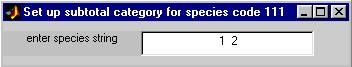
2.3.7Ā species color buttonsĀ 111-119
If you want DIGITIZER to gather statistics on a combination of two or more species as a single category, you can use one of these special species buttons to define that category.Ā If you click on one of these button, say the one just below the button labeled "110 unk24", a small sub-window will appear, in which you may type a string of species codes, for example,ĀĀ 1Ā 2ĀĀ ,ĀĀ orĀĀ 1,2ĀĀ .ĀĀ Subsequent statistics generated using the various options under the Main Window File menu will now include information derived from the superset of all samples of species 1 and species 2 combined.
2.3.8Ā species color button 120
This special species code should be used to mark samples for
special consideration, such as those that require further scrutiny or those
that are unrecognizable.Ā For this
species, lines drawn on the image are highlighted with special magenta
dots.Ā No statistics are derived for
this species code.Ā Data for this
species code may optionally be included in the histograms that are plotted and
listed using the Main Window File "write histograms" option.
2.4ĀĀĀĀĀĀ EDIT COLORMAP WINDOW
When you first import an image, it may appear washed out or too dark.Ā DIGITIZER allows you to adjust the brightness and contrast to improve visibility.Ā When you select the "edit colormap" option from the Edit pull-down menu on the Main Window, the Edit Colormap Window will appear on the screen.Ā The control in this window can be used to affect the appearance of the digitizer image in a number of ways.

The image "exposure curve", which is the relationship between the byte value of a particular pixel appearing in the image file and the screen color used to display that pixel, can also be varied in order to change the range, intensity, and contrast of the image. The overall color tint of the image can also be altered to further improve the visibility of the samples in the image.Ā
The Edit Colormap Window also displays a list of the current values of the important program parameters that are in effect for the particular samples being digitized.
2.4.1Ā graph area
shows a
plot of the relationship between the input value of a
pixel in
the image and the output value of that pixel on the display screen.ĀĀ The blue curve has three sections separated
by two blue circles.Ā You can grab a
blue circle anywhere within the plot box, use it to move the corresponding cusp
of the curve to a new location, and then press apply temp to change the
contrast and brightness of the image.
2.4.2Ā gammaĀĀĀĀĀĀĀĀĀĀĀĀĀ
enter a small number (e.g., 0.6, or 1.5) and press gamma to
change
the shape of the "exposure curve" between the two blue circles in the
graph area.
2.4.3Ā linear
click to
restore the exposure curve to a straight line between the two blue circles in
the graph area.
2.4.4Ā red, green, blue
three
editable numbers between 0 and 1 which determine the overall tint of the image
by determining the intensity levels red,
green,
and blue pixels respectively.
2.4.5Ā tint
click to show the new tint scale in the colorbar below the graph area.
2.4.6Ā save
this
saves for future digitizing sessions the current settings of all the colormap
parameters controlled by this window.
2.4.7Ā apply
click to put your parameter changes into affect.
2.4.8Ā left x, left y
the x
and y coordinates of the left blue circle.Ā
You can change each of these to an integer between 0 and 255 as an
alternative means of relocating the blue circle.
2.4.9Ā right x, right y
same as above, for the right blue circle.
2.4.10Ā undoĀĀĀ
click to restore the colormap settings to their values just prior to the most recent change you made.
2.4.11Ā reset ĀĀ
click to restore the original colormap that was in effect when the session began,Ā (If you have already saved your new values, resetĀ will not restore the original settings.)
2.4.12Ā close
click to close the Edit Colormap window
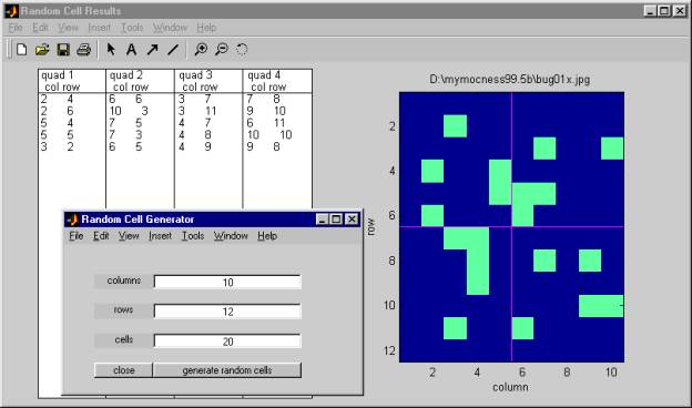
2.5ĀĀĀĀĀĀ RANDOM CELL GENERATOR WINDOW
Selecting the "generate random cells" option from the Edit pull-down menu of the Main Window creates a small window in which you can enter the approximate dimensions of the overall image (i.e., the number of cells wide vs. the number of cells high), and the number of random cells you wish to select from the overall image.
When you click on "generate random cells" in this window, the program creates another window containing a list of the cell coordinates of the randomly selected cells, together with a map of where these cells are located.
2.5.1Ā columns
enter the number of columns of cells in the overall image (rounded to an integer).
2.5.2Ā rows
enter the number of rows of cells in the overall image (rounded to an integer).
2.5.3Ā cells
enter the number of cells to be selected randomly from the total (columns X rows).
2.5.4Ā generate random cells
click here to execute the random cell generator.Ā This creates another window with the list of the selected cells and a diagram of their locations.ĀĀ The diagram is divided into approximately equal quadrants.Ā The originating image file name is used as the title of the diagram.Ā You can print the window and use it as a guide in choosing where on the image to make measurements.
2.6ĀĀĀĀĀĀ EDIT PLATE PARAMETERS WINDOW
When you select "write histograms" from the File menu of the Main Window, the program creates the Edit Plate Parameters Window shown here.Ā You use this window to enter various parameters associated with each digitized species and with the overall sample collection.Ā These parameters determine the overall calibration of the measurements, the scaling factors used for those species that were measured on only part of the image, and the histogram bin assignments.
The window is divided into several sections, each of whose controls are described in the following paragraphs.
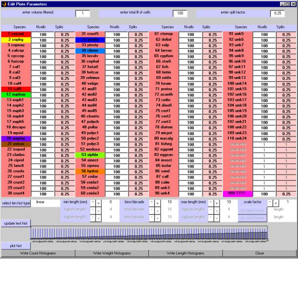
2.6.1Ā setting parameters that are common to all species
In order for DIGITIZER to produce
histograms having the proper physical units, for example, abundance data in
counts per cubic meterĀ ( 1/m^3 ), or
biomass in milligrams per cubic meterĀ (
mg/m^3 ), you must provide the program with the volume of the originating water
sample.Ā Also, if the image you used for
taking measurements was created by photographing only a fraction of the entire
water sample, you must inform the program of the "split fraction",
that is, the fraction of the total water sample you actually used to make the
image.Ā These two numbers can then be
used to convert the count and weight data derived from your measurements into
abundance (in counts per cubic meter) and biomass (in milligrams per cubic
meter).
You provide these pieces of information in the top section of the Edit Plate Parameters window which contains edit boxes for entering the values for (a) the total volume of water from which the samples were filtered, (b) the total number of grid cells that were drawn on the image when the digitizer session was initialized for this image, and (c) the "split factor".
In many cases, you may not measure
samples in all of the grid cells on a particular plate.Ā For example, there may have been so many
small copepods that you chose to measure them in only 160 of the 800 cells on a
plate.Ā In a case like this, DIGITIZER
requires that you provide the total number of cells on the plate and the number
of cells in which you actually took measurements for that particular species.
As another example, if you gathered (filtered) samples from 300 cubic meters of water, used one quarter of them to make the image, and then created an overlay grid which had 25 by 32 cells, you would enter: volume filtered ofĀ 300;Ā total number ofĀ 800Ā cells ;Ā and split factor ofĀ 0.25.ĀĀĀ The volume filtered value will then be applied to all measurements, irrespective of species.Ā The total number of cells and the split factor will also be applied to all measurements, but will be adjusted to take account of those species which were purposely NOT measured in every cell (see next section).
2.6.2Ā setting parameters that are specific to each species
The second section from the top of the Edit Plate Parameters window contains the two edit boxes for each individual species, one for the number of cells and the other for the split factor.
You can override the total number of cells by entering a specific value for the number of cells you actually used in measuring a particular species.Ā For example, if you only used 30 cells to measure small copepods (species code 1), then you would change the value in the "Ncells" box adjacent to "1 copsml" to 30.ĀĀ This will cause DIGITIZER to multiply the count and weight data for this species by the ratio of the total cells to the actual number of cells measured, in this case 300/30 = 10, before calculating statistics for small copepods.
In a similar manner, you can override the split factor that was used when measuring a particular species.Ā This might be required if you measured additional samples of a certain species using another image taken from a different portion of the total water volume filtered.Ā (This situation is not likely to occur very often.Ā The option has been provided with a future version of DIGITIZER in mind, one where measurements from multiple images can be readily combined in a single output file.)
2.6.3Ā updating the test histogram
The next lower section from the top of the Edit Plate Parameters window shows a test histogram (bar plot) that uses a simple "ramp" function to illustrate the current selection of bin parameters.Ā After adjusting one or more axis and bin selection parameters (described below), you can click on "update test histogram" to see what your bins are going to look like when you plot or print your actual data.
2.6.4Ā setting parameters that affect the plotted and printed length histograms
The third section from the top of the Edit Plate Parameters window contains several controls for specifying and previewing the bin assignments that will be subsequently used by DIGITIZER to produce printed and plotted histograms of the LENGTHS of your measurements.Ā (There is no provision in this version of DIGITIZER for making plots of WEIGHTS or COUNTS of your measurements.)
You can choose one of three means of distributing your measurements into length bins, two of which use the base10 logarithms of the lengths.Ā In each case, you can select the minimum bin boundary, the maximum bin boundary, and the overall bin spacing.
If you plan to make measurements on several images, it might be a good idea to first decide on a standard set of settings for the various binning parameters.Ā Then you can use these standard bin settings whenever you create histogram files of data from any one of your images.Ā This will make it much easier to compare histogram results derived from different images with one another.
The next few paragraphs describe the various binning options in more detail and include sample test histograms (actually, portions of the Edit Plate Parameters window) to illustrate the options.
The controls in this section of the window only affect the plots and printouts of length histograms.Ā They have no effect on weight and count histograms.
select length histogram type
This button cycles the bin assignment type among the three major choicesof bin types, as described below:
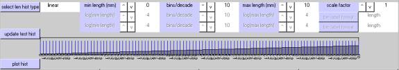
linear
This makes bins of equal width, in units of length.
The first example shows the use of linearly spaced length bins with a minimum length of zero millimeters, a maximum length of ten millimeters, and ten bins in each major length interval.Ā The overall number of bins in this case is 100 (10 x 10).Ā The axis scale factor is one.
(To reproduce the test histograms shown here and subsequently apply the same bin choices to your data, use the various button controls described below to match the settings shown.Ā Then click onĀ "update test hist".Ā Then click onĀ "plot hist".)
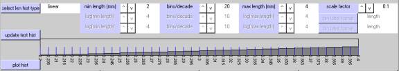
The second example of linear binning uses an axis scaling factor of 0.1, a minimum length setting of 2, a maximum length setting of 4, and a bin spacing of 20 per major length interval.Ā The minimum and maximum settings are multiplied by the scaling factor to yield a minimum length of 0.2 millimeters and a maximum length of 0.4 millimeters.Ā The total number of bins is 40 (20 x 4).
log (equal bin)
This makes bins of equal width, in units ofĀ "log-base-10-of-length".
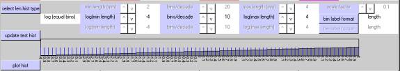
The first example uses bins based on log10(length), a minimum bin boundary of 10^-4 millimeters (0.0001 mm) and a maximum bin boundary 10^+4 millimeters (10000.0 mm).Ā Within each decade, there are 10 bins whose boundaries corresponding to the series 10^-4.0 mm, 10^-3.9 mm, 10^-3.8 mm, 10^-3.7 mm,ģ..10^+3.9 mm,Ā 10^+4.0 mm. ĀThe overall result consists of 80 bins of equal width (10 bins/decade x 8 decades), plotted on a log10 axis.
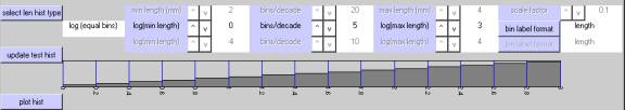
The second example uses 5 bins per decade, a minimum of 10^+0 ( 1.0 mm), and a maximum of 10^+3 (1000.0 mm).Ā In all, there are 15Ā ( 5 x 3 ) equal-width bins plotted on a log10 axis.
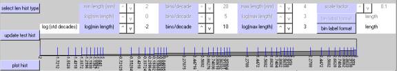
log (std decades)
This defines bins of equal width in units of length within each decade, but increases the individual bin width by a factor of 10 for each successively higher decade.Ā The results are plotted using a log base 10 axis.
(NOTE:Ā Statistics that are derived from histograms that use this binning arrangement should be interpreted cautiously, because the bin widths are not consistent across the entire range of lengths.)
The first example illustrates this alternate choice of log10 binning.Ā Here, the miniumum length is 10^-2 (0.01 mm), the maximum length is 10^+3 (1000.0 mm), and the number of bins per major interval is 10.Ā In contrast to the above examples, however, the bin boundaries within each decade correspond to the piecewise series:
ĀĀĀĀĀĀĀĀĀĀĀĀĀĀĀĀĀĀĀĀĀĀĀĀĀĀĀĀĀĀĀĀĀĀĀĀĀĀĀĀĀĀ ĀĀĀĀ Ā
log10(0.01),
log10(0.02),Ā log10(0.03),.....Ā log10(0.09),Ā log10(0.10);
log10(0.20),Ā log10(0.30),.....Ā log10(0.90),Ā log10(1.00);
log10(2.00), Ālog10(3.00),.....Ā log10(9.00),Ā
log10(10.00);
log10(20.0),Ā log10(30.0),.....Ā log10(90.0),Ā
log10(100.0).
log10(200.),Ā log10(300.),.....Ā log10(900.),Ā
log10(1000.).
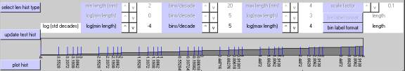
The second example uses 10^-4 mm and 10^+4 mm for the minimum and maximum bin boundaries, and 5 bins per decade.Ā The resulting bin boundaries comprise the piecewise series:
ĀĀĀĀĀĀĀĀĀĀĀĀĀĀĀĀĀĀĀĀĀĀĀĀĀĀĀĀĀĀĀĀĀĀĀĀĀĀĀĀĀĀĀĀĀĀĀĀĀĀĀĀĀĀĀĀĀĀĀĀĀĀĀĀĀĀĀĀĀĀĀĀĀĀĀĀĀĀĀĀĀĀĀĀĀĀĀĀĀĀĀĀĀĀĀĀĀ
log10(0.0001),
log10(0.0002),Ā log10(0.0004),Ā log10(0.0006),Ā log10(0.0008),Ā log10(0.0010);
log10(0.0020),Ā log10(0.0040),Ā log10(0.0060),Ā
log10(0.0080),Ā log10(0.0100);
log10(0.0200),Ā log10(0.0400),Ā log10(0.0600),Ā
log10(0.0800),Ā log10(0.1000);
log10(0.2000),Ā log10(0.4000),Ā log10(0.6000),Ā
log10(0.8000),Ā log10(1.0000).
log10(2.0000),Ā log10(4.0000),Ā log10(6.0000),Ā
log10(8.0000),Ā log10(10.000).
log10(20.000),Ā log10(40.000),Ā log10(60.000),Ā
log10(80.000),Ā log10(100.00).
log10(200.00),Ā log10(400.00),Ā log10(600.00),Ā
log10(800.00),Ā log10(1000.0).
log10(2000.0),Ā log10(4000.0),Ā log10(6000.0),Ā
log10(8000.0),Ā log10(10000.).
For each axis type, you can cycle through a number of numeric choices using theĀ "^ " (up) and "v" (down) buttons associated with each option.Ā The "bins/decade" cycles from 1 to 20.Ā The choices for the other parameters vary, but the upper bin limit is constrained to be greater than the lower bin limit.
The controls are:
min length
Sets
the lower bin limit.
max length
Sets
the upper bin limit.
bins/decade
Sets
the number of bins in each decade (group of 10 bins).
scale factor
For the linear binning option,
this sets a multiplier for the lower and upper bin limits.
bin label format
For the two log binning options, this determines how the bins will be labeled in the left hand column of the histogram output spreadsheet data.Ā Click on the "bin label format" button to cycle through these three options:
ĀĀĀĀĀĀĀĀĀĀĀĀĀĀĀĀĀĀĀĀĀĀĀ lengthĀĀĀĀĀĀĀĀĀĀĀĀĀĀ histogram rows labeled by length
ĀĀĀĀĀĀĀĀĀĀĀĀĀĀĀĀĀĀĀĀĀĀĀ log(length)ĀĀĀĀĀĀĀ histogram rows labeled by log(length)
ĀĀĀĀĀĀĀĀĀĀĀĀĀĀĀĀĀĀĀĀĀĀĀ len,log(len)ĀĀĀĀĀĀĀ histogram rows labeled by both length
and log(length)
The results of this option show up only in the histogram output files, not in the histogram plots.
2.6.5Ā making a histogram plot
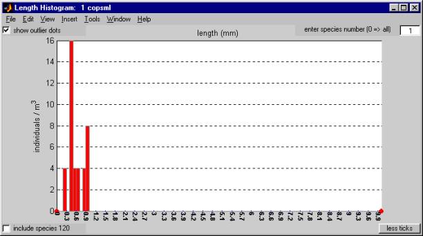
To get a histogram plot of your real data, click on the "plot hist" button near the bottom left corner of the window.Ā This creates a Length Histogram window containing a histogram plot of your data, binned according to sample length.
The Length Histogram window has several controls for selecting the species and adjusting the tick mark labels.
ĀĀĀĀĀĀĀĀĀĀĀ enter species number (0 => all):
To plot a particular species, enter its species code in the edit box in the upper right corner of the window.Ā A species code ofĀ 0 will result in a histogram based on the lengths of all the species combined.
include species 120:
Samples represented by the "special" species code "999 ????"Ā will not beĀ included in this histogram unless the "include species 120" checkbox is marked.
show outlier dots:
The counts of outliers, that is, samples whose lengths are less that the bin minimum or greater than the bin maximum, are designated by red dots at the edges of the plot.Ā If you un-check the "show outlier dots" checkbox, these dots will not be shown.
You can print the histogram plot by using the print option of the File menu at the top of the Length Histogram window.ĀĀ The controls boxes in the window will be included on the plot, but they don't look very good on certain printers.
NOTE:Ā If you are very careful you can enter a series of statements in the MATLAB command window which will temporarily hide the controls on the plot so that the printed copy will look better.Ā These statements involve identifying the MATLAB "graphics object handles" for the GUI controls on the plot, and then disabling their "visibility" properties.
If you want to do this, here's how:
(1) Click on the top of the Length Histogram window to make it the last active MATLAB figure.
(2) Click DIRECTLY on the MATLAB Command Window.Ā (Don't click on any other MATLAB figure or the next statement won't work properly.)
(3) Key in these MATLAB statements:
>> gcf
(This should return the number 55. If it does not, repeat steps 1 and 2 until it does.)
>> ixxxx = findobj(gcf,'type','uicontrol')
>> set(ixxxx,'vis','off')
(4)Ā Now use the print option of the File menu at the top of the Length Histogram window to print the histogram.
(5)Ā To restore the control boxes on the plot, use the MATLAB Command Window to keyin:
>> set(ixxxx,'vis','on')
2.6.6Ā writing a histogram file
At the bottom of the Edit Plate Parameters window are buttons for creating ASCII files containing the histogram data.Ā Each button brings up an appropriate file selection window in which you can specify a destination directory and filename.Ā DIGITIZER then writes a text file which is easily imported into the EXCEL spreadsheet program.Ā (The files look peculiar when listed as pure text because they are" blank-delimited" in order to make the EXCEL importing step more robust.)
In the case of the "Write length histogram" button, the data in the text file should exactly match the data in the length histogram plot (described above).
There is a significant difference
between the bins boundaries that are used for length histograms, and those that
are used for either count or weight histograms.Ā For the length histograms that use logarithmic bins, the
logarithms are base 10 logarithms.
In contrast, the count and weight
histograms both employ traditional "octave" binning according to
weight class.Ā Octave binning uses bin
boundaries that increase successively by factors of two, with an occasional
rounding off to avoid cumbersome fractions.Ā
(This binning arrangement may be thought of as logarithm base 2 binning,
ignoring the slight discontinuities at the roundoff points).
Thus, DIGITIZER's octave binning
scheme employs the following sequence of bin boundaries:
0.000008,Ā 0.000016,Ā
0.000032,Ā 0.000064,Ā 0.000128,Ā
0.000256,Ā 0.000512,
ĀĀĀ (round off the next value fromĀĀ 0.001024ĀĀĀ toĀĀĀ 0.001000)
0.001,Ā 0.002,Ā 0.004,Ā 0.008,Ā
0.016,Ā 0.032,Ā 0.064,Ā
0.128,Ā 0.256,Ā 0.512,
ĀĀĀ (round off the next value fromĀĀ 1.024ĀĀĀ toĀĀĀ 1.000)
1,Ā 2,Ā 4,Ā 8,Ā
16,Ā 32,Ā 64,Ā
128,Ā 256,Ā 512,
ĀĀĀ (round off the next value fromĀĀ 1024ĀĀĀ toĀĀĀ 1000)
1000,Ā 2000.
2.6.7Ā closing the window
The Close button closes the Edit Plate Parameter window and the Length Histogram window.
3ĀĀĀĀĀĀĀĀĀ TUTORIALS
The tutorial exercises assume that you have already installed MATLAB and know something about how to use it.Ā They also assume that you know how to use Microsoft Windows, and that you have installed and are somewhat familiar with Microsoft EXCEL.
Here's how to install DIGITIZER.
STEP1:Ā Copy ONE of the program folders from the distribution CD to your hard disk.Ā The choice depends on which version of Windows and which version of MATLAB you are using.
For Windows 98 and MATLAB 6.1, copy folderĀ dig100w98m61Ā from CD to hard disk.
For Windows 98 and MATLAB 6.5, copy folderĀ dig100w98m65Ā from CD to hard disk.
For Windows 2000 and MATLAB 6.1, copy folderĀ dig100w2000m61Ā from CD to hard disk.
For Windows 2000 and MATLAB 6.5, copy folderĀ dig100w2000m65Ā from CD to hard disk.
STEP 2:Ā Change the name of the resulting hard disk folder toĀ dig100.
STEP 3:Ā Copy the tutorial folderĀ tut100ĀĀ from the distribution CD to hard disk.
STEP 4:Ā IMPORTANT:Ā Change the disk access properties of both folders and all the files in them to READ/WRITE access, by un-checking their "Read-only" Attributes.Ā Here's how to do this:
In My Computer or Windows Explorer, select the file(s) or folder(s) whose disk access property(s) you want to change.
(You can select multiple files or folders by using the shift key in the customary Windows manner:Ā click on the first file in the contiguous list of files or folders to be selected; then hold down the shift key and click on the last file in the contiguous list of files or folders to be selected.)
On the File menu, click Properties.
(You can also right-click a folder or file on your desktop, and then click Properties.)
Un-check the "Read-only" checkbox in the Properties dialog box and click OK.
The tutorials below assume that you have copied the folders to hard drive D.
You can change the folder names if you wish, but don't change any file names.
IMPORTANT: Please note that the default.men and default.wgt files must be located in the æworking directoryÆ along with the image file in order for DIGITIZER to run.
3.1ĀĀĀĀĀĀ TUTORIALĀ 1
This tutorial shows you how to start DIGITIZER, how to add a few new measurements to an existing output file that already contains several previous measurements, how to save your results, and how to import your results into an EXCEL spreadsheet.
Using Windows Explorer or some other file copying method of your preference, make a copy of the file tutorial.matĀ and call itĀ mytutorial.mat.
(You should do this at the start of any exercise that uses the tutorial.matĀ file, for example, Tutorial 3.Ā If you forget, you can always restore the original tutorial.matĀ file from the distribution medium.)
Start MATLAB and at the prompt ( >> )Ā keyin:
ĀĀĀĀĀĀĀĀĀĀĀ >>cdĀ d:\tut100 ;
ĀĀĀĀĀĀĀĀĀĀĀ >>path(Ā 'd:\dig100' , pathĀ ) ;
ĀĀĀĀĀĀĀĀĀĀĀ >>digitizer
(You can instead add the tutorial path with the File/Set Path menu option in the MATLAB Command Window.)
Close the Copyright window, or wait a few seconds for it to disappear.
3.1.1Ā Select the input and output files
In the input file selection window, enterĀĀ *.jpgĀ in the file name box , and double click on fileĀ tutorial.jpg.Ā (This window may be hidden behind other windows, so you might have to click on its icon on the Windows taskbar.)
In the Job Type message box, select "Existing".
In the output file selection window, double click on the fileĀ mytutorial.mat.
The Main Window should now display an image of a digitized sample plate. Superimposed on the image are a reference grid and several colored lines indicating organisms that have already been measured.Ā You are now ready to measure some more organisms.
3.1.2Ā Add your own measurements
Enter the numbers 5 and 2 in the "column" and "row" edit boxes respectively, and then click onĀ "select a cell" .
Click on "zoom out" to change the display to include the nine cells centered on cell 5-2.
Click on "2 coplrg" to indicate that you are going to measure large copepods.
Click on the upper end of the large copepod in cell 6-1.Ā Then click on the lower end of the same copepod that is in cell 6-2.Ā See Appendix 1 for measurement guidelines.
A yellow line with X's at the ends should appear on the image, and the MATLAB Command Window should display information regarding the measurement (sample number, species number, length, calculated weight, cell location, plate name, and split factor).
If you change your mind part way through the measurement, you can click on the "undo pending" button in the Main Window and then begin the measurement over again.Ā To try this, click on one end of a copepod, but stop before you click on the other end.Ā Now click on "undo pending" to cancel the effect of the partial measurement you have just made.
In a similar manner, measure the large copepod in cell 4-1.
Now pan to cell 6-4 using theĀ " v", "^", ">", and "<"buttons until it is in the center of the display and then click onĀ "zoom in".
Click on the "1 copsml" button so that you can now measure small copepods.
Successively click on both ends of several small copepods.Ā Each successful measurement should result in a red line on the image.
Pull down the Main Window File Menu and select "SAVE DATA and continue".
This writes your measurements to two separate files:
the MATLAB-formatted (non-printable) file namedĀĀ "mytutorial.mat" ĀĀ which you chose when you started the program, and
a text-formatted (printable) file namedĀĀ mytutorial.datĀĀ which is given the same name as the .mat file but with the file extension .dat .
The older versions of these two files are replaced.
List the contents of the text file in the command window by entering
ĀĀĀĀĀĀĀĀĀĀĀ >>typeĀ mytutorial.dat
3.1.3Ā Print statistics
From the Main Window File Menu selectĀ "write statistics", and in the resulting output file selection window enter "stats1" to create an output statistics file.
Use EXCEL to open and examine stats1.txt, as follows:
ĀĀĀĀĀĀĀĀĀĀĀ Start
EXCEL.
ĀĀĀĀĀĀĀĀĀĀĀ OpenĀ stats1.txt.
ĀĀĀĀĀĀĀĀĀĀĀ Choose
"Delimited", and click "Next".
ĀĀĀĀĀĀĀĀĀĀĀ ChooseĀ Delimiters:ĀĀ "Space", and click "Next".
ĀĀĀĀĀĀĀĀĀĀĀ Click "Finish".
(You can also examineĀ "stats1.txt" with your favor text editor, but the file is difficult to read because it is blank delimited and therefore not well collimated.)
3.1.4Ā Save you results and quit DIGITIZER
In DIGITIZER, from the FILE Menu select "SAVE DATA and quit" and confirm the selection by clicking on "Yes".Ā This will update your output data files, terminate DIGITIZER, and exit MATLAB.
3.2ĀĀĀĀĀĀ TUTORIALĀ 2
This tutorial shows you how to start a new digitizing session on a new sample plate, how to tailor the appearance of the Main Window and its image to your liking, and how to make measurements of samples along curved lines.
As you did in the previous tutorial, start MATLAB, change directories, update the path, and start DIGITIZERĀ (see Section 3.1).
Again, selectĀĀ tutorial.jpgĀĀ in the input file selection window.
This time, click on "New" in the Job Type message box.
Enter a new filenameĀĀ mytutorial2.matĀĀ in the output file selection box and click
on "save".
Select the fileĀĀ alternate.menĀĀ from the menu file selection window and
click on "save".
3.2.1Ā Initialize the calibration parameters and image reference grid:
In the blue edit boxes in the upper right corner of the Main Window, replace the default text items with the following:
plate:ĀĀĀĀĀĀĀĀĀĀĀĀĀĀĀ tutorial 2
split:ĀĀĀĀĀĀĀĀĀĀĀĀĀĀĀĀ 0.25
xoff(pix):ĀĀĀĀĀĀĀĀĀĀ 10
yoff(pix):ĀĀĀĀĀĀĀĀĀĀ 20
pix/inch:ĀĀĀĀĀĀĀĀĀĀĀ 1200
cm/cell:
ĀĀĀĀĀĀĀĀĀĀĀ 1.0
Click on "set
parameters" to observe the reference grid on the image.
(You can repeat these steps if you
make a mistake.)
Click on "OK TO START" to
accept these settings, and then click on "YES" in the resulting
WARNING message box to make these choices permanent.
3.2.2Ā Edit the colormap of the image to improve its contrast.
Choose the "edit colormap
option from the MainWindow Edit menu to bring up theĀ "Edit Colormap" window.
In this window, using the left
mouse button and the cursor, drag the upper right hand blue circle in the white
plot area to the approximate coordinates 110,160.Ā This changes the "exposure curve" (a photographic term)
in the color bar directly below the plot area.
(You may
have to grab the circle by its bottom half because the cursor is not active if
it is outside the white plot area.)Ā
Alternatively, you could have
entered the numbers 110 and 160 in the right x and right y edit boxes
respectively, and then clicked on "linear" update the colorbar.
Click on the "apply" button to make the new exposure curve take effect on the actual image.
Change the tint of the image from pale green to rose by entering 1,Ā 0.9, andĀ 0.9Ā in the red, green, and blue edit boxes respectively, clicking on "tint" and then clicking on "apply"
(If you don't like the revised
exposure curve or the new tint, click onĀĀ
reset.)
Click on the "save" button to make
these changes permanent.
Click on the "close" button to
close the Edit Colormap window.
3.2.3Ā Change the allowable length limits for a
species
Try to measure a large copepod.Ā You should hear a beep and get an error message in the command window informing you that the measurement was too long.Ā This has probably occurs because the minimum and maximum legal lengths for large copepods are set incorrectly.
To change these settings, select the "Edit Species Buttons, Lengths,... " option from the Main Window menu.
This creates the "Species Parameter" window which shows the current settings for the legal length minima and maxima.
Click on the yellow "2 coplrg" to create a "Set Length Limits ..." window.
In this window, enter 2.5 and 10 in the minimum and maximum edit boxes respectively.
Click on "apply length changes".
Click on "save length changes".
While you are at it, change the length limits for small copepods as well.Ā First click on the red "1 copsml" button in the "Edit Species" window.Ā Then change the small copepod limits to 0.1 to 2.4999, click on "apply length changes", and then click on "save length changes".
Click on the X in the upper right corner of the "Edit Species Parameters" window to close the two windows.
Now you can measure large and small copepods correctly.
3.2.4Ā Make some measurements using theĀ 2-pointĀ mode
To select and enlarge a sub-region
of the image, first click on the "manual zoom on" button in the Main
Window.Ā This changes the function of
the cursor from measuring to zoom control.
Using the left mouse button,
stretch out a rectangular box on the image that encloses several copepods.Ā (To do this, place the cursor on the upper
left corner of the desired area, press and hold the left mouse button, drag the
cursor to the lower right corner of the desired area, and release the mouse
button.)
Click on the "manual zoom
off" button.Ā This changes the
function of the cursor back to measuring.
Click on the "2 coplrg" species
button and measure several large copepods (see Section 3.1.2).Ā Click on the "1 coplrg" species button and
measure several small copepods.
Click on "refresh screen" in the Main Window to cause DIGITIZER to redraw the entire Main Window.Ā (Refreshing the screen may be necessary in certain circumstances, often when a point or line is removed from the image.Ā "refresh screen" puts DIGITIZER, MATLAB, the Windows operating system, the video driver and display, and so forth, back in step with each other.)
3.2.5Ā Add a species button to the main menu and change its properties
Now you are going to
measure the euphausiid in cells 7-8,Ā 8-8,Ā
and 9-8.Ā For increased accuracy,
you would like to measure it along a curved line rather than along a straight
line.Ā To make this measurement, you
first have to do several things:
add theĀ "12 euphau" Ā species button to the main menu,
change the "12 euphau" Ā
button color (so you can see the measurements better),
change the maximum and minimum allowable lengths for
euphausiids,
use the new species button to select euphausiids, and
temporarily switch DIGITIZER to n-point mode.
To accomplish these items, do the following:
Select the "Edit Species Buttons, Lengths,..." option from the Main Window Edit menu to brings up theĀ "Species Parameter" window.
Click on theĀ "12 euphau" Ā button to create a "Set Length Limits" Window.
Make the following changes to the entries:
Check
the box labeled "show on main window" in the top left corner,
Change
the red, green , and blue edit boxes to 1,Ā
0.75, andĀ 0Ā respectively, and
Click
onĀĀ "apply color/visibility changes".
Change
the min and max length edit boxes to 1 and 100 respectively, and
Click
onĀ "apply length changes"
A gold coloredĀ ō12 euphauöĀĀ button should now be included on the Main Window, and the
allowed limits for euphausiids should now be listed asĀ 1Ā
andĀ 100Ā in theĀĀ
Species Parameters Window.
In theĀ "Set Length Limits"ĀĀ window, click onĀĀ "save length changes"ĀĀ to make the length limit changes permanent.
In the "Set Length Limits"ĀĀ window, click onĀĀ "save color/visibility changes"ĀĀ to make the new button color and its appearance on the Main Window permanent.ĀĀ
Click on the X in the upper right corner of the "Species Parameters Window" to close the windows.
On the Main Window, click onĀĀ "12 euphau".
You are now ready to
measure euphausiids.
3.2.6Ā Measure a curved specimen using theĀ "n-point"Ā mode
Pan and/or zoom to the nine cells
centered on cell 8-8.
Click on the button labeled
"n-pt" to switch mode for measuring along curved lines.
Place the cursor on one end of the
specimen, click and HOLD DOWN the left mouse button while tracing the cursor
from one end of the organism to the other end.Ā
Release the mouse button at the other end of the specimen. (If you want
to make a lot of successive n-point measurements, use the n-point digitizing
mode option in the Main Window Preferences menu to the select "n-pt
persistent" setting.Ā Then you
won't have to click on "n-pt" before each measurement.)
It takes a little practice to
measure curved organisms smoothly.Ā The
first few times you try to use n-point mode, you may want to delete the curve
and try again.Ā In the next tutorial,
you will learn how to delete measurements.
3.2.7ĀĀ Save your results and quit DIGITIZER
From the FILE Menu select "SAVE DATA and quit" and confirm the selection by clicking on "Yes".Ā This will update your output data files, terminate DIGITIZER, and exit MATLAB.
3.3ĀĀĀĀĀĀ TUTORIALĀ 3
This
tutorial shows you how to delete an unwanted measurement, how to change the
species designation of a measurement that was originally categorized
incorrectly, and how to use the species buttonĀ
"999 ????"Ā to mark an
item (such as an unknown specimen) for later consideration.
Start a new DIGITIZER session as
you did in Tutorial 1Ā (see Sections 3.1
and 3.1.1).
Measure a lot of specimens of
various species without worrying about whether or not you have made
mistakesĀ (see Section 3.1.2)
SelectĀ "SAVE DATA and continue" Ā
from the Main Window File menu to update your output files.
Now perform the steps in the
following sections (in any order) to get the feel how DIGITIZER lets you edit
and remove samples and from your output files.
3.3.1Ā Remove measurements using select by cursor
Click on the button labeled
"select by cursor".
Position the cursor over one of
the colored lines on the image that represents a digitized sample, and click
the left mouse button to highlight the sample.
Click on "delete
selection" to remove that measurement from the screen.
3.3.2Ā Change the species code of a measurement using select by number
Click on theĀ "show sample numbers"Ā button under Main Window View menu to
display the sample numbers on the screen.Ā
(If the numbers on the screen are too big, use the Main Window View
optionĀĀ "change sample number
size"ĀĀ to choose a smaller font.)
Click the button labeledĀ "select by number", and enter a
sample number such as "3" in the white edit box that appears above
theĀĀ select by numberĀĀ button and press the "enter"Ā key on the keyboard.Ā Sample number 3 should be highlighted by a
white dotted line.Ā The image should
automatically zoom in to the cell containing sample number 3.
Click on "cancel
selection" to keep the measurement because you have changed your mind and
decided not to delete sample 3 after all.
Click on "select by
number" again, and enter aĀ "
4" in the edit box to highlight sample number 4 on the image.
Click on the "change
species" button.Ā The status
message box should display "WAITING FOR SPEC CODE".
Click on the tan colored species
selection button labeledĀ "7
cal1"Ā on the Main Window to change
sample 4Ā from species 1 to species 7.
At this point the program will
check to see if the lengths of the selected samples comply with the legal
length limits for the newly assigned species 7.Ā If they do not comply, the error messageĀĀ "One or more samples was deleted
because its length was illegal"ĀĀ
will appear in a message box, and the non-complying sample(s) will be
deleted from the image and from the output files.
3.3.3Ā Delete multiple measurements at once using select by region
Zoom out to see a larger portion
of the image.
Click on "select by
region".
With the left mouse button,
stretch out a rectangular region on the image that surrounds three or four
samples.Ā A red rectangle should appear
on the image, and a message box labeled "Select species within the red
box" should appear on the screen.
If you don't like your choice of a
selected region, click on "CANCEL" in the message box and repeat the above
step.
Otherwise, click on "ALL" in the
message box to select all the samples within the red rectangle.
(For details on which samples are
considered to be within the rectangle, see "region selection
criteria" in the Preferences Menu section of the documentation.).
Click on "delete
selection".Ā AĀ "WATCH OUT!!!"Ā message box should appear warning you that
you are about to delete several measurements.Ā
There is currently no way to "undo" this operation, so be sure
you've selected the right samples.)
3.3.4Ā Delete specimens of a single species using select by region
Click on "select by
region" again, stretch out another red rectangle around a few more
measurements, click on "ALL" the resulting message box, and then click on
"cancel selection" in the Main Window to undo the entire selection.
Click on "select by region"
again and stretch out another red rectangle that surrounds a few more
measurements, this time including at least one small copepod (species code 1).
Now click on "ONE" in the
resulting message box.
This should change the status
message to "PRESS A SPECIES BUTTON".
Next, click on the "1
copsml" button on the Main Window to highlight only the small copepods
inside the red rectangle.
Finally, click on "delete
selection" to remove these measurement(s) from the image.
3.3.5Ā Change species codes for several specimens at once using select by region
Click on "select by
region" and stretch out a red rectangle on the image surrounding several
sample of different species.
Select "ALL" in the "Select
species" message box.
Click on the "change
species"Ā button on the Main
Window.
The status message should change
to "WAITING FOR SPECIES CODE".
Click on the species button
"7 cal1".
A "WATCH OUT!!!" message
box should appear.Ā Accept the changes
by clicking on YES.
(At this point, you may get
another WARNING message box informing you that one or more measurements have
been deleted.ĀĀĀ This occurs whenever a
selected sample has a length that is legal for its original species code but is
not legal for its new species code.)
To change the species codes of a
SINGLE species within a selected region, again select by region, stretch out a
red rectangle surrounding several measurements.
This time, click on "ONE" in the
"Select species" message box.
Pick out a specimen in the red box
that has already been measured, and whose species designation you wish to
change.Ā First click on the species
button in the Main Window that corresponds to specimen you have picked out.
This should highlight your specimen on the image, along with any other
specimens within the red box also have this species designation.
Next, click on "change
species".
Finally, click on the new
(correct) species button in the Main Window, and confirm the change in the
WARNING message box.
This procedure does several things
for each of the altered specimens:Ā On
the image, it redraws each specimen in a new color; it recalculates the weight
of each specimen using the new species weight formula; it discards any specimen
whose length no longer lies within the new species length limits; it rewrites
theĀĀ .matĀĀ andĀĀ .datĀĀ output data files in order to replace the
old data with the new data.
3.3.6Ā Mark unknown specimens
Click on the 999 ???? button.
Go to cell 8-2 on the image and measure the diameter of the circular "thing" (actually a bubble) in the upper left corner of the cell.
Similarly, go to cell 8-8 and draw a circle abound the "blob" of specimens.Ā Use n-point mode by first clicking on n-pt and then tracing a line around the blob.
Click on "show all
cells" in the Main Window to display the entire image so you can get a
better look at how these "unknowns" are displayed.
3.3.7Ā Save your results and quit DIGITIZER
From the FILE Menu select "SAVE DATA and quit" and confirm the selection by clicking on "Yes".Ā This will update your output data files, terminate DIGITIZER, and exit MATLAB.
3.4ĀĀĀĀĀĀ TUTORIALĀ 4
This TutorialĀ familiarizes you with some of the program output options.
Start MATLAB and DIGITIZER as you
did in Tutorial 1 (see Sections 3.1 and 3.1.1).
3.4.1Ā Create an output statistics file
Select the Main Window File
"write statistics" menu item, and enter the output filenameĀ "stats1"Ā in the Select Statistics Spreadsheet File window.
(You already did this in Tutorial
1 so in the resulting warning message box you will have to allow the program to
overwrite your older stats1.txt file.)
Examine the file with EXCEL.
3.4.2Ā Create output length and weight files
Select the Main Window File
"write lengths" menu item, and enter the output filenameĀ "length1" in the Select Statistics
Spreadsheet File window.
Select the Main Window File
"write weights" menu item, and enter the output filenameĀ "weight1" in the Select Statistics
Spreadsheet File window.
Examine the results using EXCEL.
3.4.3Ā Create a histogram plot of the measured sample lengths
Select "write histograms" from the File Menu.Ā This creates the "Edit Plate Parameters" window.
At the top of the window, enter the volume filtered,Ā total number of cells, and split factor edit boxes with the values 100,Ā 64,Ā andĀ 0.25 respectively.
Click on "plot hist" in the lower left corner to create a histogram plot.
To plot the bars for small copepods only, change the species code in the upper right edit box from 0 to 1 and press the "enter" key on the keyboard.
(If you want to improve the appearance of the plot and then print it, see the Edit Plate Parameters window options described in Section 2.6).
3.4.4Ā Create a histogram file of the measured sample lengths
At the bottom of the "Edit Plate Parameters" window, click on "Write Length Histograms", and enter the filename "lenhist1" in the resulting file selection window.
Examine the output file using EXCEL.
The data in the spreadsheet should match the data represented by the bars in the above histogram plot.
3.4.5Ā Create a histogram file of the counts of the measured samples
In the same Edit Plate Window, click on "Write Count Histograms" to produce a text formatted histogram file of the measured sample counts (the species abundance data).
Examine the output file using EXCEL.
3.4.6Ā Create a histogram file of the weights of the measured samples
In the same Edit Plate Window, click on "Write Weight
Histograms" to produce a text formatted histogram file of the measured sample
weights.
Examine the output file using EXCEL.
3.4.7Ā Save you results and quit DIGITIZER
From the FILE Menu select "SAVE DATA and restart".Ā This will update your output data files, but instead of terminating DIGITIZER, and exiting MATLAB, the program will reset itself so that you can immediately begin a new session.
(If you wish to quit this DIGITIZER session instead of proceeding to Tutorial 5, just selectĀ "cancel" in the image file selection window and then click on "Abort" in the message box to exit DIGITIZER. Otherwise, proceed to Tutorial 5.)
3.5ĀĀĀĀĀĀ TUTORIALĀ 5
This tutorial shows you how to select a random subset of the cells in yourĀ image.Ā It describes how to customize the input file that determines the appearance of the Main Window.ĀĀ It tells how to change the input file that contains the formulas for calculating sample weights.
If you are just starting a new DIGITIZER session, start MATLAB and DIGITIZER as you did in Tutorial 1 (see Sections 3.1 and 3.1.1).
If, on the other hand, you are continuing directly from Tutorial 4 above, just select the image fileĀ tutorial.jpgĀ and existing data fileĀ mytutorial.matĀ as you did in Tutorial 1 (that is, skip over Section 3.1 and just do Section 3.1.1).
3.5.1Ā Selecting Random Cells
Assume you only want to make
measurements of small copepods in some of the cells of the image because there
are all together too many small copepods.
From the Edit Menu, choose
"generate random cells".
In the edit boxes of the resulting
Random Cell Generator Window, enter the approximate number of columns and rows
of cells on the image, and the number of cells you want to have in the
subset.Ā In this case, enter 8, 8, and
10 respectively.Ā
Click onĀ "generate random cells"Ā to create a list of randomly chosen cells and a diagram of where
they are on the image.
(Note that cells are chosen in
equal numbers from the four approximately equal quadrants of the image, and
that the number chosen is rounded up to a multiple of four.)
Use the Print option in the File
menu of the Random Cells Results window to make a hard copy of the results so
that you can use it as a guide in selecting cells in which to measure small
copepods .
Now measure all of the small
copepods that lie within the chosen cells.Ā
SelectĀĀ "SAVE DATA and continue" ĀĀ
from the File menu of the Main Window.
3.5.2Ā Making a new species file
Use the Species Parameters Window from the Main/Edit/edit species menu to add a few species buttons to the Main Window.
Make the changes permanent, and close the Species Parameters Window (see Section 3.2.5).
From the Main Window File Menu, selectĀ "Save species file as... "
In the resulting output file specification window, enter a new file name with the file extension .men, for example, enter "mymenu.men".
Save and quit DIGITIZER (see Section 3.2.7).
The next time you use DIGITIZER and you choose to create a new output file, your newly generated menu file "mymenu.men" will appear as one of the choices.
3.5.3Ā Making a new weights file
There are currently no graphical user interface (GUI) controls for modifying the contents of the fileĀ default.wgtĀĀ which contains the weight formulas used by DIGITIZER.Ā Therefore, change or add a weight formula, you must VERY CAREFULLY use a text editor such as Wordpad, or the built-in MATLAB editor, as described here.
Make a backup copy ofĀ default.wgtĀĀ (!!).ĀĀ Call it default_backup.wgt.
Display the MATLAB editor window (for example, by keying inĀ >>editĀ if necessary).
Open the file default.wgt
To REPLACE an existing weight formula, locate the formula to be replaced by searching for the appropriate species number in column one.
Change the formula in the THIRD FIELD of the record with the new formula which:ĀĀĀ
(a) must be a legitimate MATLAB
arithmetic expression,
(b) must use the capital letter L
for the independent variable "length",Ā and
(c) must contain NO BLANKS (or
other white space).
To ADD a weight formula to the file because one does not yet exist for a particular species, add a new line anywhere after the first record of the file.Ā The new line must have precisely the same fields as the other lines in the file.Ā The fields are:
species code,
one or more blanks,
the name of the species WITH ALL BLANKS (or white space) REPLACED BY UNDERSCORES,
one or more blanks,
the formula with NO BLANKS or white space, as described above.
DIGITIZER will not read theĀ default.wgtĀ file correctly if it contains spurious white spaces (blanks, tabs, carriage returns, etc.)
Save the modifiedĀ default.wgt file for later use.
3.5.4Ā Changing the weights file during a session
Ordinarily, the weight formulas used by DIGITIZER will be the ones that were in effect when the output .mat file for a particular plate was first created.Ā If you wish to change or add a weight formula after that point and have it take affect immediately, you must do the following.
Create a new weight file that contains the change or addition, as described in the previous section, BUT name it something other than default.wgt, for example "newweights.wgt"
Then, selectĀ "Read Alternate Weight File" from the Main Window File Menu.
ChooseĀ "newweights.wgt"Ā from the input file selection window.
The revised weight formula(s) will affect future measurements on this plate, but will not change the weights which were calculated and saved for measurements made previously.Ā
To RETROACTIVELY change the calculated weights of all past measurements using the new weight formula(s), use the steps in the next section.
3.5.5Ā Recalculating the weights of existing measurements.
If you want all past as well as
future measurements on this plate to use the revised weight formula(s),
selectĀĀ "Recalculate sample
weights"Ā from the MainWindow File
menu.
Click on "Yes" in the two
successive WARNING message boxes.
Some of your previous plots and spreadsheets (or else the new ones) are probably wrong!
3.5.6Ā Save you results and quit DIGITIZER
From the FILE Menu select "SAVE DATA and quit" and confirm the selection by clicking on "Yes".Ā This will update your output data files, terminate DIGITIZER, and exit MATLAB.
4ĀĀĀĀĀĀĀĀĀ SYSTEM REQUIREMENTS AND RESTRICTIONS
DIGITIZER was written and tested in MATLAB 6.1 and 6.5.Ā It employs a MATLAB Graphical User Interface (GUI) so that nearly all program operations are controlled by means of the mouse and the cursor on the display screen.Ā The program has been tested on Windows 98 and Windows 2000 PCs.
DIGITIZER requires at least 512
Mbytes of main memory, and preferably 1 Gbyte.Ā
There must be sufficient memory for a scanned image, plus approximately
10 Mbytes for the MATLAB program and the stored measurements.
There must also be adequate disk
space for the MATLAB source code, the original input image file, and several
output data files, including a 6.6 Mbyte ".mat"Ā file of output data and a 6.6 MbyteĀ .mbkĀ
backup file.
5ĀĀĀĀĀĀĀĀĀ KNOWN PROBLEMS
There is currently a graphics
interface problem when running DIGITIZER under MATLAB 6.5.Ā Before running DIGITIZER, you must un-select
all of MATLAB View Menu options except the Command Window to avoid a conflict
between certain internal MATLAB/JAVA resources and the DIGITIZER Edit Species
Parameters Window.
There are speed degradation
problems when running DIGITIZER under MATLAB 6.1, particularly when a large
number of samples have been digitizer.Ā
Resizing a window, for example, may take several seconds.Ā These problems are apparently caused by
inefficient use of OpenGL graphics utilities employed by MATLAB 6.1, and have
been fixed in MATLAB 6.5.
Nearly the entire DIGITIZER program files (m-files and p-files) are MATLAB scripts, rather than MATLAB functions.Ā These scripts all operate in the main MATLAB workspace, one consequence of which is that all of the program variables may be observed or changed (peeked or poked) in the MATLAB command window by you, the user.Ā Therefore, you are strongly advised not to do anything else in the MATLAB command window besides watch the DIGITIZER status and error messages.
The data files used by DIGITIZER must be writeable as well as readable, that is, they must NOT be Read Only files.Ā Under some circumstances, when you archive DIGITIZER files to a CD ROM, for example, and then later restore them to hard disk,Ā the files will acquire Read Only status.Ā When you try to run DIGITIZER, you will go merrily along until you digitize the twentieth specimen or so, at which point you will get an obscure file related-error message (which seems to vary depending upon the exact circumstances).Ā If this sort of thing happens, check to see if your DIGITIZER files on hard disk are Read Only.Ā If they are, use the appropriate WINDOWS utility to make them Read/Write files and see if the problem goes away.
When EXCEL imports length histogram data files, the row label for the lowest bin boundary appears as a spreadsheet entryĀ "#NAME?",Ā whereas it should appear as the textĀ "-Infy" (minus infinity).Ā To eliminate this problem, when importing a length histogram text file into EXCEL, change the Column Data Format of column 1 from "General" to "Text".Ā
6ĀĀĀĀĀĀĀĀĀ SOFTWARE ON CD-ROM AND THE WEB
The files on the CD-ROM included with this technical report allow you to install DIGITIZER version 1.0 on Windows 98 or Windows 2000 (it also works, but has not been thoroughly tested, on Windows XP).Ā The folders contains 'p files' for Matlab versions 6.1 and 6.5.
See "TUTORIALS" in this Handbook for instructions on installing the program and associated files.
Contents of CD-ROM.:
dig100w98m61dig100w98m65
dig100w2000m61
dig100w2000m65
tut100Ā - tutorial files, including default menu and weights files
Files may also be downloaded from:
ftp://globec.whoi.edu/pub/software/digi_prog/WHOI_Silhouette_DIGITIZER.htm
-or go to http://globec.whoi.edu/globec.html and follow the path to Program Documentation / software tools/ DIGITIZER.
Appendix 1ĀĀĀĀ Standard Lengths Used in DIGITIZER Program
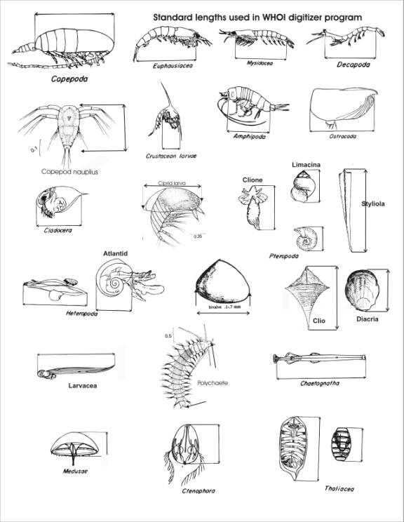
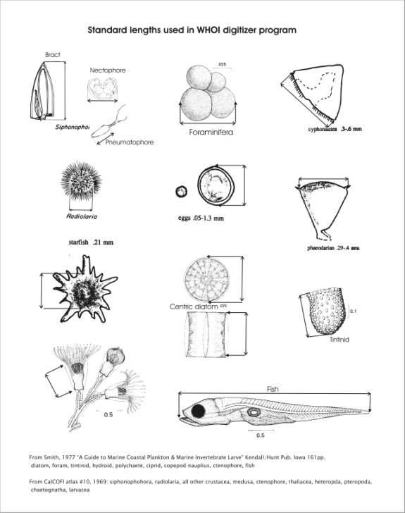
Appendix 2ĀĀĀĀ Length to Wet Weight Biomass Conversion Formulas.Ā
L in the formula is the length
(mm) as described in the figures shown above.
R means a regression of length
(mm) and weights (mg) was derived from a population of animals.
V means the formula is based on
the shape of the organism and a density of 1 was assumed.Ā This was used for rare or very small
animals.