This example demonstrates the functions in the Bioinformatics Toolbox for working with Affymetrix GeneChip data.
Note that the affyread function is only supported on Microsoft Windows.
The function affyread can read four types of Affymetrix data files. These are DAT files, which contain raw image data, CEL files that contain information about the expression levels of the individual probes, CHP files that contain information about probe sets, and EXP files which contain information about experimental conditions and protocols. affyread can also read CDF and GIN library files. The CDF file contains information about which probes belong to which probe set and the GIN file contains information about the probe sets such as the gene name with which the probe set is associated. To learn more about the actual files, you can download sample data files from: http://www.affymetrix.com/support/technical/sample_data/demo_data.affx
The raw image data from chip scanner is saved in the DAT file. If you use affyread to read a DAT file you will see that it creates a MATLAB structure.
datStruct = affyread('Drosophila-121502.dat')
datStruct =
               Name: 'Drosophila-121502.DAT'
           DataPath: 'd:\affydata'
            LibPath: 'd:\affydata'
       FullPathName: 'd:\affydata\Drosophila-121502.DAT'
           ChipType: 'DrosGenome1'
               Date: 'Jan 07 2003 12:20PM'
    NumPixelsPerRow: 4733
            NumRows: 4733
            MinData: 0
            MaxData: 20804
          PixelSize: 3
         CellMargin: 2
          ScanSpeed: 17
           ScanDate: 'Nov 14 2000 07:35AM'
          ScannerID: ''
         UpperLeftX: 225
         UpperLeftY: 234
        UpperRightX: 4491
        UpperRightY: 238
         LowerLeftX: 227
         LowerLeftY: 4499
        LowerRightX: 4492
        LowerRightY: 4503
         ServerName: ''
              Image: [4733x4733 uint16]
Fields of the structure can be accessed using the dot notation.
datStruct.NumRows
ans =
        4733
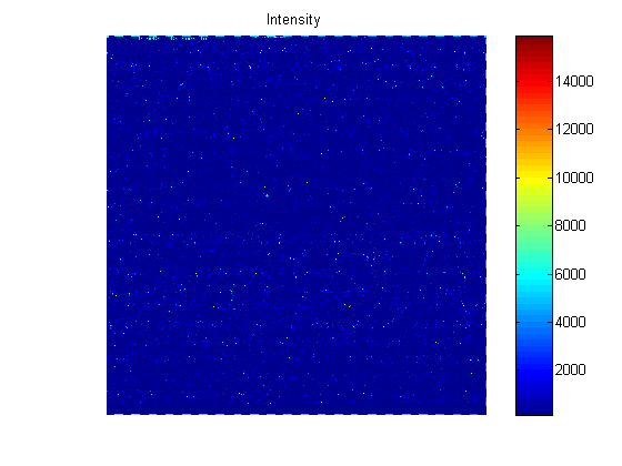
The imagesc command can be used to display the image.
datFigure = figure;
imagesc(datStruct.Image);
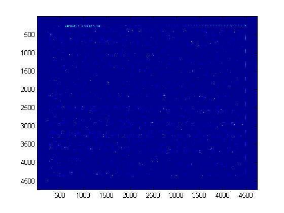
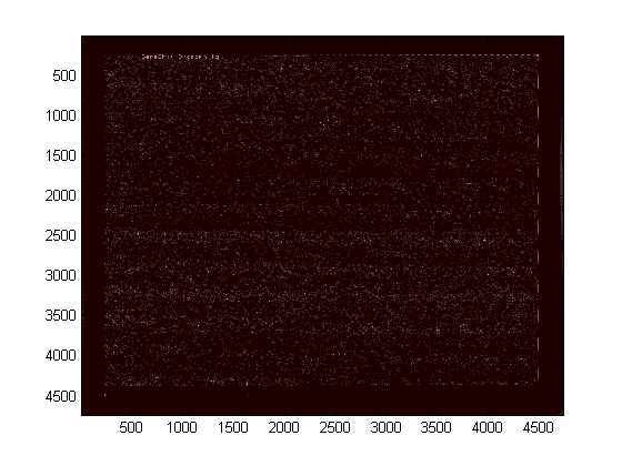
You can change the colormap from the default jet to another using the colormap command.
colormap pink
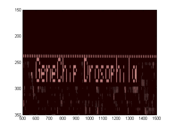
You can zoom in on a particular area with the mouse, or with the axis command. Notice that this stretches the y-axis.
axis([500 1500 150 350])
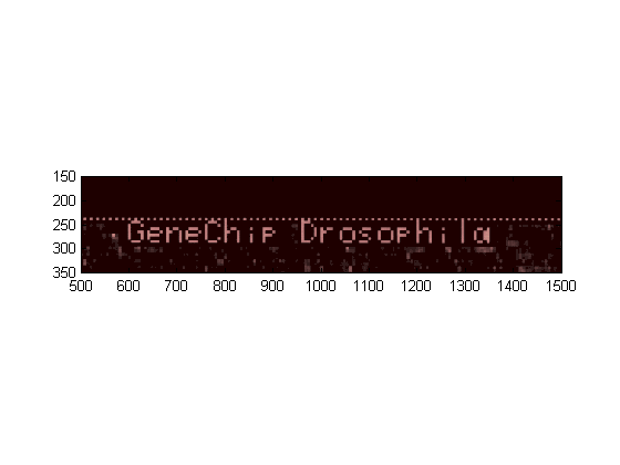
You can force the axes to be equal using the axis image command.
axis image
axis([500 1500 150 350])
The information about each probe on the chip is extracted from the image data by the Affymetrix image analysis software. The information is stored in the CEL file. affyread reads a CEL file into a structure. Notice that many of the fields are the same as those in the DAT structure.
celStruct = affyread('Drosophila-121502.cel')
celStruct =
                Name: 'Drosophila-121502.CEL'
            DataPath: 'd:\affydata'
             LibPath: 'd:\affydata'
        FullPathName: 'd:\affydata\Drosophila-121502.CEL'
            ChipType: 'DrosGenome1'
                Date: 'Jun 19 2002 02:04PM'
         FileVersion: 3
           Algorithm: 'Percentile'
           AlgParams: [1x61 char]
        NumAlgParams: 4
          CellMargin: 2
                Rows: 640
                Cols: 640
           NumMasked: 0
         NumOutliers: 485
           NumProbes: 409600
          UpperLeftX: 225
          UpperLeftY: 234
         UpperRightX: 4491
         UpperRightY: 238
          LowerLeftX: 227
          LowerLeftY: 4499
         LowerRightX: 4492
         LowerRightY: 4503
          ServerName: ''
    ProbeColumnNames: {8x1 cell}
              Probes: [409600x8 double]
The CEL file contains information about where each probe is on the chip and also the intensity values for the probe. You can use the maimage function to display the chip.
celFigure = figure;
maimage(celStruct)
Again, you can zoom in on a specific region.
axis([30 200 0 25])
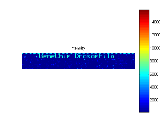
If you compare the image created from the CEL file and the image created from the DAT file, you will notice that the CEL image is lower resolution. This is because there is only one pixel per probe in this image, whereas the DAT file image has many pixels per probe.
The structures created by affyread can be very large. It is a good idea to clear them from memory once they are no longer needed.
clear datStruct
close(datFigure);
The Probes field of the CEL structure contains information about the individual probes. There are eight values per probe. These are stored in the ProbeColumnNames field of the structure.
celStruct.ProbeColumnNames
ans =
    'PosX'
    'PosY'
    'Intensity'
    'StdDev'
    'Pixels'
    'Outlier'
    'Masked'
    'ProbeType'
So if look at one row of the Probes field of the CEL structure you will see eight values corresponding to the X position, Y position, intensity, and so forth.
celStruct.Probes(1,:)
ans =
  Columns 1 through 7
         0         0  120.0000   88.3000   25.0000         0         0
  Column 8
    1.0000
The probe set information in the CEL file by itself is not particularly useful as there is no indication in the file as to which probe set a probe belongs. This information is stored in the CDF library file associated with a chip type. The CDF files are typically stored in a central library directory.
% libDir is the directory for the library files.
libDir = 'D:\Affymetrix\LibFiles\DrosGenome1';
cdfStruct = affyread('DrosGenome1.cdf',libDir)
cdfStruct =
               ChipType: 'DrosGenome1'
                LibPath: 'D:\Affymetrix\LibFiles\DrosGenome1'
           FullPathName: 'D:\Affymetrix\LibFiles\DrosGenome1\DrosGenome1.CDF'
                   Date: 'Aug 27 2004 10:47AM'
                   Rows: 640
                   Cols: 640
           NumProbeSets: 14010
         NumQCProbeSets: 13
    ProbeSetColumnNames: {6x1 cell}
              ProbeSets: [14023x1 struct]
Most of the information in the file is about the probe sets. In this example there are 14010 regular probe sets and 13 QC probe sets. The ProbeSets field of the structure is a 14023 array of structures.
cdfStruct.ProbeSets
ans =
14023x1 struct array with fields:
    Name
    ProbeSetType
    CompDataExists
    NumPairs
    NumQCProbes
    QCType
    ProbePairs
A probe set record contains information about the name, type and number of probe pairs in the probe set.
cdfStruct.ProbeSets(100)
ans =
              Name: '142176_at'
      ProbeSetType: 'Regular'
    CompDataExists: 0
          NumPairs: 14
       NumQCProbes: 0
            QCType: 0
        ProbePairs: [14x6 double]
The information about where the probes for a probe set are on the chip is stored in the ProbePairs field. This is a matrix with one row for each probe pair and six columns. The information in the columns corresponds to the ProbeSetColumnNames of the CDF structure.
cdfStruct.ProbeSetColumnNames
cdfStruct.ProbeSets(100).ProbePairs(1,:)
ans =
    'ProbeSetNumber'
    'ProbePairNumber'
    'PMPosX'
    'PMPosY'
    'MMPosX'
    'MMPosY'
ans =
        1056           0         271         369         271         370
The first column shows the probe set ID number, the second column, the probe pair number is 0. This is because Affymetrix uses zero based indexing for their probe numbering. The remaining columns give the X and Y coordinates of the PM and MM probes on the chip. You can use these coordinates to look up the values for a probe from the celStruct
PMX = cdfStruct.ProbeSets(100).ProbePairs(1,3);
PMY = cdfStruct.ProbeSets(100).ProbePairs(1,4);
theProbe = find((celStruct.Probes(:,1) == PMX) & ...
                       (celStruct.Probes(:,2) == PMY))
theProbe =
      236432
You can then extract all the information about this probe from the CEL structure.
celStruct.Probes(theProbe,:)
ans =
  Columns 1 through 7
  271.0000  369.0000  193.3000   23.8000   20.0000         0         0
  Column 8
    1.0000
If you want to do this lookup for all probes, you can use the function probelibraryinfo. This creates a matrix with one row per probe and three columns. The first column is index of the probe set to which the probe belongs. The second column contains the probe pair index and the third column indicates if the probe is a perfect match (1) or mismatch (-1) probe. Notice that index of the probe pair index is 1 based.
probeinfo = probelibraryinfo(celStruct,cdfStruct);

probeinfo(theProbe,:)
ans =
   100     1     1
The function probesetvalues does the reverse of this lookup and creates a matrix of information from the CEL and CDF structures containing all the information about a given probe set. This matrix has 18 columns corresponding to ProbeSetNumber, ProbePairNumber, UseProbePair, Background, PMPosX, PMPosY, PMIntensity, PMStdDev, PMPixels, PMOutlier, PMMasked, MMPosX, MMPosY, MMIntensity, MMStdDev, MMPixels, MMOutlier, and MMMasked.
psvals = probesetvalues(celStruct,cdfStruct,'142176_at')
psvals =
  Columns 1 through 7
   99.0000         0         0         0  271.0000  369.0000  193.3000
   99.0000    1.0000         0         0  316.0000  261.0000   54.3000
   99.0000    2.0000         0         0  373.0000  545.0000  568.0000
   99.0000    3.0000         0         0  126.0000   49.0000  444.0000
   99.0000    4.0000         0         0  192.0000   39.0000  158.0000
   99.0000    5.0000         0         0  579.0000  381.0000   60.0000
   99.0000    6.0000         0         0  199.0000   75.0000  297.0000
   99.0000    7.0000         0         0  166.0000   33.0000  219.0000
   99.0000    8.0000         0         0   74.0000  605.0000  277.0000
   99.0000    9.0000         0         0    1.0000   19.0000  182.0000
   99.0000   10.0000         0         0  269.0000  339.0000   64.0000
   99.0000   11.0000         0         0  127.0000  569.0000  130.0000
   99.0000   12.0000         0         0  112.0000  259.0000  512.0000
   99.0000   13.0000         0         0  475.0000  103.0000  213.3000
  Columns 8 through 14
   23.8000   20.0000         0         0  271.0000  370.0000   72.0000
   12.7000   20.0000         0         0  316.0000  262.0000   48.0000
   60.4000   25.0000         0         0  373.0000  546.0000  446.0000
   38.3000   25.0000         0         0  126.0000   50.0000  497.0000
   23.4000   25.0000         0         0  192.0000   40.0000  107.8000
    9.8000   25.0000         0         0  579.0000  382.0000   51.0000
   37.1000   25.0000         0         0  199.0000   76.0000  222.0000
   53.5000   25.0000         0         0  166.0000   34.0000  126.0000
  120.1000   25.0000         0         0   74.0000  606.0000  127.0000
   19.5000   16.0000         0         0    1.0000   20.0000  152.5000
    9.4000   25.0000         0         0  269.0000  340.0000   51.0000
   25.3000   20.0000         0         0  127.0000  570.0000   66.0000
   67.9000   25.0000         0         0  112.0000  260.0000  519.0000
   21.3000   20.0000         0         0  475.0000  104.0000  140.0000
  Columns 15 through 18
   14.2000   20.0000         0         0
    9.8000   25.0000         0         0
   49.2000   20.0000         0         0
   58.2000   25.0000         0         0
   14.3000   20.0000         0         0
   10.1000   25.0000         0         0
   49.3000   25.0000         0         0
   19.9000   20.0000         0         0
   14.6000   25.0000         0         0
   15.4000   20.0000         0         0
    9.0000   25.0000         0         0
   12.5000   25.0000         0         0
   44.7000   20.0000         0         0
   35.5000   25.0000         0         0
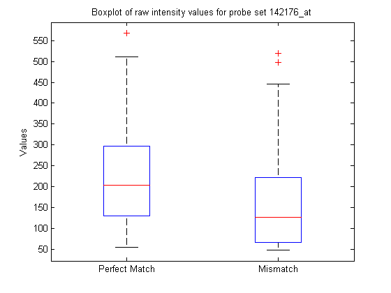
You can extract the intensity values from the matrix and look at some of the statistics of the data.
pmIntensity = psvals(:,7);
mmIntensity = psvals(:,14);
boxplot([pmIntensity,mmIntensity],'labels',{'Perfect Match','Mismatch'})
title('Boxplot of raw intensity values for probe set 142176_at',...
    'interpreter','none')
% Use interpreter none to prevent the TeX interpreter treating the _ as
% subscript.
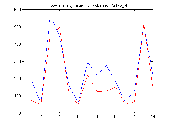
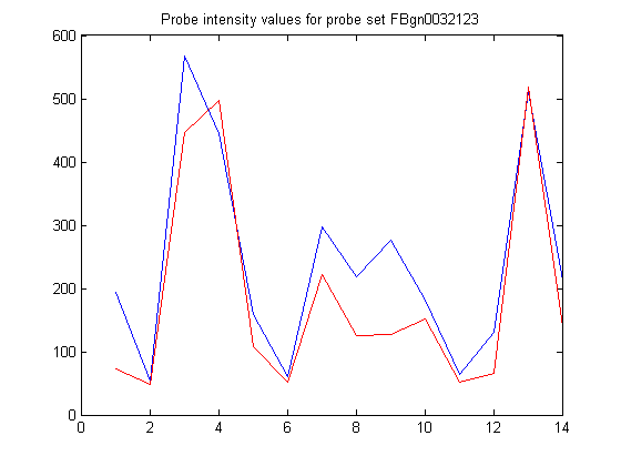
Or plot the values for the individual probes.
figure
plot(pmIntensity,'b'); hold on
plot(mmIntensity,'r'); hold off
title('Probe intensity values for probe set 142176_at',...
    'interpreter','none')
The Affymetrix probe set IDs are not particularly descriptive. The mapping between the IDs and the gene names is stored in the GIN file. This is a text file so you can open it in an editor and browse through the file, or you can use affyread to read the information into a structure.
ginStruct = affyread('DrosGenome1.gin',libDir)
ginStruct =
            Name: 'DrosGenome1'
         Version: 2
    ProbeSetName: {14010x1 cell}
              ID: {14010x1 cell}
     Description: {14010x1 cell}
     SourceNames: {3x1 cell}
       SourceURL: {3x1 cell}
        SourceID: [14010x1 double]
You can search through the structure for a particular probe set. Alternatively, you can use the function probesetlookup to find out information the gene name for a probe set.
info = probesetlookup(cdfStruct,'142176_at')
info =
      Identifier: 'FBgn0032123'
    ProbeSetName: '142176_at'
        CDFIndex: 100
        GINIndex: 1021
     Description: [1x140 char]
          Source: 'Flybase'
       SourceURL: [1x58 char]
You can use the Identifier field to add the gene name to the plot title.
newTitle = sprintf('Probe intensity values for probe set %s',...
                                                        info.Identifier);
title(newTitle)
The output from probesetlookup includes a link to the source web site for the gene associated with a probe set.
web(info.SourceURL,'-browser')
The function probesetlink will link out to the NetAffx web site to show the actual sequences used for the probes. Note that you will need to be a registered user of NetAffx to access this information.
probesetlink(cdfStruct,'142176_at');
The CHP file contains the results of the experiment. These include the average signal measures for each probe set as determined by the Affymetrix software and information about which probe sets are called as present, absent or marginal and the p-values for these calls.
chpStruct = affyread('Drosophila-121502.chp',libDir)
chpStruct =
                   Name: 'Drosophila-121502.CHP'
               DataPath: 'd:\affydata'
                LibPath: 'D:\Affymetrix\LibFiles\DrosGenome1'
           FullPathName: 'd:\affydata\Drosophila-121502.CHP'
               ChipType: 'DrosGenome1'
                   Date: 'Jun 19 2002 02:17PM'
               CellFile: 'c:\genechip\testdata\arraycd\Drosophila.CEL'
              Algorithm: 'ExpressionStat'
                AlgType: 2
            AlgTypeName: 'Statistical'
             AlgVersion: '5.0'
           NumAlgParams: 13
              AlgParams: [1x157 char]
         NumChipSummary: 3
            ChipSummary: [1x10² char]
                   Rows: 640
                   Cols: 640
           NumProbeSets: 14010
         NumQCProbeSets: 13
    ProbeSetColumnNames: {18x1 cell}
             ServerName: ''
              ProbeSets: [14023x1 struct]
The ProbeSets field contains information about the probe sets. This includes some of the library information similar such as the ID and the type of probe set, and also results information such as the calculated signal value and the preset/absent/marginal call information. The call is given in the 'Detection' field of the ProbeSets structure. The '142176_at' probe set is called as being 'Present'.
chpStruct.ProbeSets(100)
ans =
                     Name: '142176_at'
             ProbeSetType: 'STAT'
           CompDataExists: 0
                 NumPairs: 14
             NumPairsUsed: 14
                   Signal: 817.0113
                Detection: 'Present'
          DetectionPValue: 0.0014
              CommonPairs: 0
           SignalLogRatio: []
        SignalLogRatioLow: []
       SignalLogRatioHigh: []
                   Change: []
             ChangePValue: []
                 Positive: []
                 Negative: []
    NumPairsUsedInAvgDiff: []
         PositiveFraction: []
               LogAverage: []
              PosNegRatio: []
        AverageDifference: []
             AbsoluteCall: []
                 Increase: []
                 Decrease: []
            IncreaseRatio: []
            DecreaseRatio: []
           PositiveChange: []
           NegativeChange: []
              IncDecRatio: []
        DPosDNegDiffRatio: []
        LogAvgRatioChange: []
            AvgDiffChange: []
         BaselineIsAbsent: []
               FoldChange: []
                SortScore: []
           DifferenceCall: []
              NumQCProbes: 0
                   QCType: 0
               ProbePairs: [14x18 double]
However, the '142177_at' probe set is called 'Absent'.
chpStruct.ProbeSets(101)
ans =
                     Name: '142177_at'
             ProbeSetType: 'STAT'
           CompDataExists: 0
                 NumPairs: 14
             NumPairsUsed: 14
                   Signal: 68.1834
                Detection: 'Absent'
          DetectionPValue: 0.4130
              CommonPairs: 0
           SignalLogRatio: []
        SignalLogRatioLow: []
       SignalLogRatioHigh: []
                   Change: []
             ChangePValue: []
                 Positive: []
                 Negative: []
    NumPairsUsedInAvgDiff: []
         PositiveFraction: []
               LogAverage: []
              PosNegRatio: []
        AverageDifference: []
             AbsoluteCall: []
                 Increase: []
                 Decrease: []
            IncreaseRatio: []
            DecreaseRatio: []
           PositiveChange: []
           NegativeChange: []
              IncDecRatio: []
        DPosDNegDiffRatio: []
        LogAvgRatioChange: []
            AvgDiffChange: []
         BaselineIsAbsent: []
               FoldChange: []
                SortScore: []
           DifferenceCall: []
              NumQCProbes: 0
                   QCType: 0
               ProbePairs: [14x18 double]
You can calculate how many probe sets are called as being 'Present',
numPresent = sum(strcmp('Present',{chpStruct.ProbeSets.Detection}))
numPresent =
        6066
'Absent',
numAbsent = sum(strcmp('Absent',{chpStruct.ProbeSets.Detection}))
numAbsent =
        7476
and 'Marginal'.
numMarginal = sum(strcmp('Marginal',{chpStruct.ProbeSets.Detection}))
numMarginal =
   468
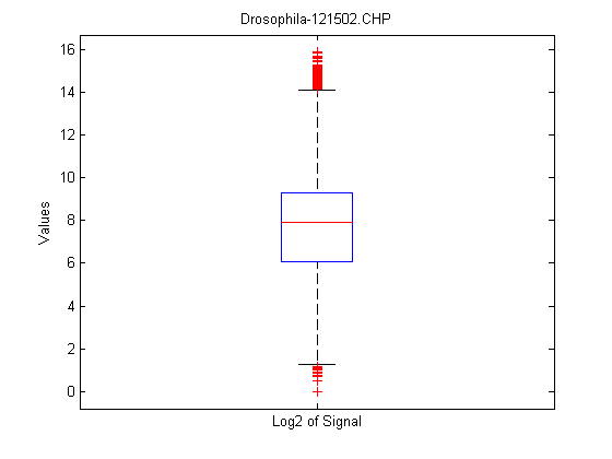
maboxplot will display a box plot of the log2 signal values for all probe sets.
maboxplot(chpStruct,'Signal','title',chpStruct.Name)
The CHP structure also contains information about the probe values for the probe set. These results are generally the same as the information created by the probesetvalues function though there are some differences. The major difference is that the intensity values in the probe pair values are normalized, and some of the placeholder columns for the probesetinfo results are populated.
chpVals = chpStruct.ProbeSets(info.CDFIndex).ProbePairs(1,:)
chpVals =
  1.0e+003 *
  Columns 1 through 7
         0         0    0.0020    0.4431    0.2710    0.3690    2.0483
  Columns 8 through 14
    0.0238    0.0200         0         0    0.2710    0.3700    0.7630
  Columns 15 through 18
    0.0142    0.0200         0         0
Compare these with the psvals from the probesetvalues. Notice the normalization factor in the seventh and fourteenth columns.
% Some of the psvals are zero so disable the divide by zero warning.

ws = warning('off','MATLAB:divideByZero');
chpVals./psvals(1,:)
warning(ws);
ans =
  Columns 1 through 7
         0       NaN       Inf       Inf    1.0000    1.0000   10.5965
  Columns 8 through 14
    1.0000    1.0000       NaN       NaN    1.0000    1.0000   10.5965
  Columns 15 through 18
    1.0000    1.0000       NaN       NaN
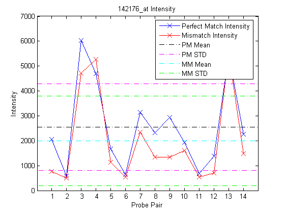
The function probesetplot creates a plot of the probes in a probe set from the CHP structure. The showstats option adds the mean, and lines for +/- one standard deviation for both the perfect match and the mismatch probes to the plot.
figure
probesetplot(chpStruct,'142176_at','showstats',true);
Affymetrix, GeneChip, and NetAffx are registered trademarks of Affymetrix, Inc.