Extracts some sequences from GenBank, shows how to find open reading frames (ORFs), and then aligns the sequences using global and local alignment algorithms.
The Help Browser can be utilized to explore the web; for example, you can view the NCBI web site (http://www.ncbi.nlm.nih.gov/) from within MATLAB.
web('http://www.ncbi.nlm.nih.gov/')
One of the many fascinating parts of the NCBI web site is the "Genes and diseases" section. This section provides a comprehensive introduction to medical genetics.
web('http://www.ncbi.nlm.nih.gov/books/bv.fcgi?call=bv.View..ShowSection&rid=gnd')
In this demonstration you will be looking at genes associated with Tay-Sachs Disease.
web('http://www.ncbi.nlm.nih.gov/books/bv.fcgi?call=bv.View..ShowSection&rid=gnd.section.220')
Tay-Sachs is an autosomal recessive disease caused by mutations in both alleles of a gene (HEXA, which codes for the alpha subunit of hexosaminidase A) on chromosome 15. The NCBI reference sequence for HEXA has accession number NM_000520.
web('http://www.ncbi.nlm.nih.gov/entrez/viewer.fcgi?val=13128865&db=Nucleotide&dopt=GenBank')
You can use the getgenbank function to read the sequence information into MATLAB.
humanHEXA = getgenbank('NM_000520')
humanHEXA =
                LocusName: 'NM_000520'
      LocusSequenceLength: '2255'
     LocusNumberofStrands: ''
            LocusTopology: 'linear'
        LocusMoleculeType: 'mRNA'
     LocusGenBankDivision: 'PRI'
    LocusModificationDate: '26-OCT-2004'
               Definition: [1x63 char]
                Accession: 'NM_000520'
                  Version: 'NM_000520.2'
                       GI: '13128865'
                 Keywords: []
                  Segment: []
                   Source: 'Homo sapiens (human)'
           SourceOrganism: [3x65 char]
                Reference: {1x11 cell}
                  Comment: [15x67 char]
                 Features: [59x74 char]
                      CDS: [1x1 struct]
                 Sequence: [1x2255 char]
                SearchURL: [1x10⁸ char]
              RetrieveURL: [1x97 char]
By doing a BLAST search or by searching in the mouse genome you will find that AK080777 is a mouse hexosaminidase A gene.
mouseHEXA = getgenbank('AK080777')
mouseHEXA =
                LocusName: 'AK080777'
      LocusSequenceLength: '1839'
     LocusNumberofStrands: ''
            LocusTopology: 'linear'
        LocusMoleculeType: 'mRNA'
     LocusGenBankDivision: 'HTC'
    LocusModificationDate: '03-APR-2004'
               Definition: [1x150 char]
                Accession: 'AK080777'
                  Version: 'AK080777.1'
                       GI: '26348756'
                 Keywords: 'HTC; CAP trapper.'
                  Segment: []
                   Source: 'Mus musculus (house mouse)'
           SourceOrganism: [3x66 char]
                Reference: {1x6 cell}
                  Comment: [12x66 char]
                 Features: [32x74 char]
                      CDS: [1x1 struct]
                 Sequence: [1x1839 char]
                SearchURL: [1x10⁷ char]
              RetrieveURL: [1x97 char]
If you don't have a live web connection, you can load the data from a MAT-file using the command
%load hexosaminidase % <== Uncomment this if no live connection
You can use the function seqshoworfs to look for ORFs in the sequence for the human HEXA gene. Notice that the longest ORF is on the third reading frame. The output value in the variable 'humanORFs' is a structure giving the position of the start and stop codons for all the ORFs on each reading frame.
humanORFs = seqshoworfs(humanHEXA.Sequence)
humanORFs =
1x3 struct array with fields:
    Start
    Stop
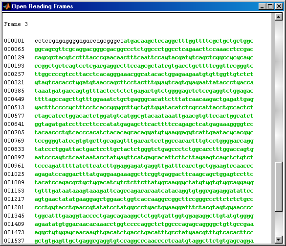
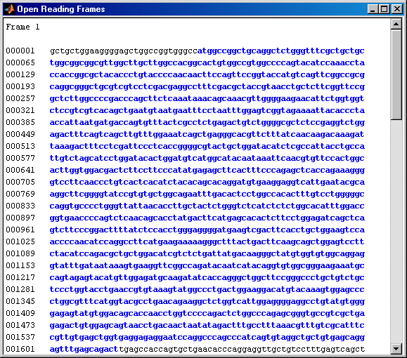
Now look at the ORFs in the mouse HEXA gene. In this case the ORF is on frame 1.
mouseORFs = seqshoworfs(mouseHEXA.Sequence)
mouseORFs =
1x3 struct array with fields:
    Start
    Stop
The first step is to use global sequence alignment to look for similarities between these sequences. You could look at the alignment between the nucleotide sequences but it is generally more instructive to look at the alignment between the protein sequences. So the first thing that you need to do is to convert the nucleotide sequences into the corresponding amino acid sequences. Use the nt2aa function to do this.
mouseProtein = nt2aa(mouseHEXA.Sequence);
Remember that the human HEXA gene was on the third reading frame, so you need to tell the function which frame to use.
humanProtein = nt2aa(humanHEXA.Sequence,'Frame',3);
One of the easiest ways to look for similarity between sequences is with a dot plot.
seqdotplot(humanProtein,mouseProtein)
ylabel('Human hexosaminidase A');xlabel('Mouse hexosaminidase A');
Warning: Match matrix has more points than available screen pixels.
         Scaling image by factors of 1 in X and 2 in Y
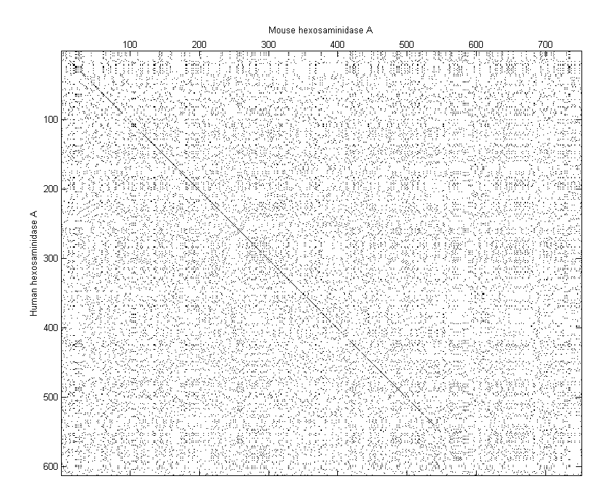
With the default settings, the dot plot is a little difficult to interpret, so you can try a slightly more stringent dot plot.
seqdotplot(humanProtein,mouseProtein,4,3)
ylabel('Human hexosaminidase A');xlabel('Mouse hexosaminidase A');
Warning: Match matrix has more points than available screen pixels.
         Scaling image by factors of 1 in X and 2 in Y
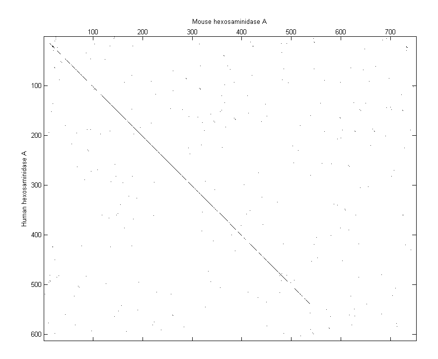
The diagonal line indicates that there is probably a good alignment so you can now take a look at the global alignment using the function nwalign which uses the Needleman-Wunsch algorithm.
[score, globalAlignment] = nwalign(humanProtein,mouseProtein);
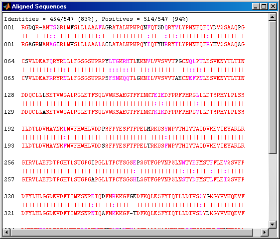
The function showalignment displays the alignment in the Help Browser with matching and similar residues highlighted in different colors.
showalignment(globalAlignment);
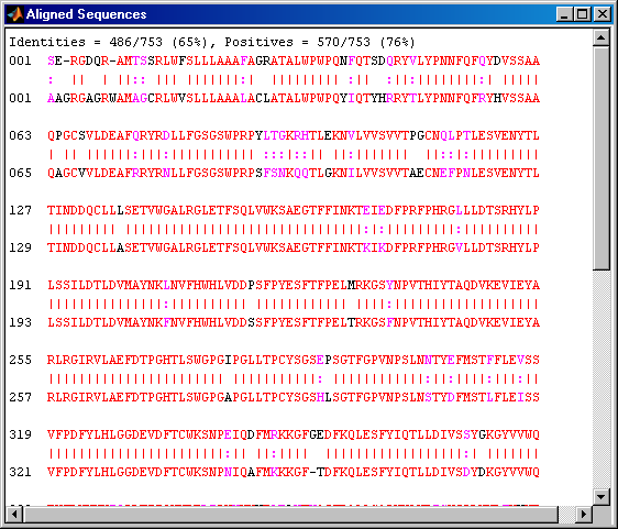
The alignment is very good for the first 540 nucleotides after which the two sequences appear to be unrelated. Notice that there is a STOP () in the sequence at this point. If the sequence is shortened so that only the regions up until the STOPs are considered, then it seems likely that you will get a better alignment. Use the *find command to look for the indices of the STOPs in the sequence.
humanStops = find(humanProtein == '*')
mouseStops = find(mouseProtein == '*')
humanStops =
   538   550   652   661   669
mouseStops =
   539   557   574   606
Use these indices to truncate the sequences at the STOPs.
humanSeq = humanProtein(1:humanStops(1));
humanSeqFormatted = seqdisp(humanSeq)
mouseSeq = mouseProtein(1:mouseStops(1));
mouseSeqFormatted = seqdisp(mouseSeq)
humanSeqFormatted =
  1  SERGDQRAMT SSRLWFSLLL AAAFAGRATA LWPWPQNFQT SDQRYVLYPN NFQFQYDVSS
 61  AAQPGCSVLD EAFQRYRDLL FGSGSWPRPY LTGKRHTLEK NVLVVSVVTP GCNQLPTLES
121  VENYTLTIND DQCLLLSETV WGALRGLETF SQLVWKSAEG TFFINKTEIE DFPRFPHRGL
181  LLDTSRHYLP LSSILDTLDV MAYNKLNVFH WHLVDDPSFP YESFTFPELM RKGSYNPVTH
241  IYTAQDVKEV IEYARLRGIR VLAEFDTPGH TLSWGPGIPG LLTPCYSGSE PSGTFGPVNP
301  SLNNTYEFMS TFFLEVSSVF PDFYLHLGGD EVDFTCWKSN PEIQDFMRKK GFGEDFKQLE
361  SFYIQTLLDI VSSYGKGYVV WQEVFDNKVK IQPDTIIQVW REDIPVNYMK ELELVTKAGF
421  RALLSAPWYL NRISYGPDWK DFYVVEPLAF EGTPEQKALV IGGEACMWGE YVDNTNLVPR
481  LWPRAGAVAE RLWSNKLTSD LTFAYERLSH FRCELLRRGV QAQPLNVGFC EQEFEQT*
mouseSeqFormatted =
  1  AAGRGAGRWA MAGCRLWVSL LLAAALACLA TALWPWPQYI QTYHRRYTLY PNNFQFRYHV
 61  SSAAQAGCVV LDEAFRRYRN LLFGSGSWPR PSFSNKQQTL GKNILVVSVV TAECNEFPNL
121  ESVENYTLTI NDDQCLLASE TVWGALRGLE TFSQLVWKSA EGTFFINKTK IKDFPRFPHR
181  GVLLDTSRHY LPLSSILDTL DVMAYNKFNV FHWHLVDDSS FPYESFTFPE LTRKGSFNPV
241  THIYTAQDVK EVIEYARLRG IRVLAEFDTP GHTLSWGPGA PGLLTPCYSG SHLSGTFGPV
301  NPSLNSTYDF MSTLFLEISS VFPDFYLHLG GDEVDFTCWK SNPNIQAFMK KKGFTDFKQL
361  ESFYIQTLLD IVSDYDKGYV VWQEVFDNKV KVRPDTIIQV WREEMPVEYM LEMQDITRAG
421  FRALLSAPWY LNRVKYGPDW KDMYKVEPLA FHGTPEQKAL VIGGEACMWG EYVDSTNLVP
481  RLWPRAGAVA ERLWSSNLTT NIDFAFKRLS HFRCELVRRG IQAQPISVGC CEQEFEQT*
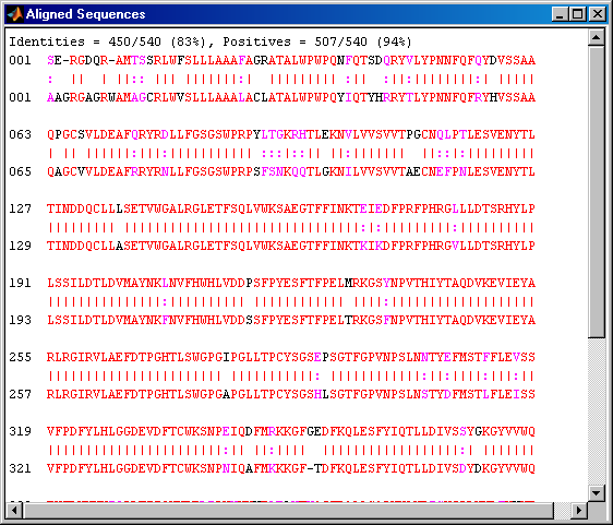
If you align these two sequences and then view them you will see a very good global alignment.
[score, alignment] = nwalign(humanSeq,mouseSeq);
showalignment(alignment);
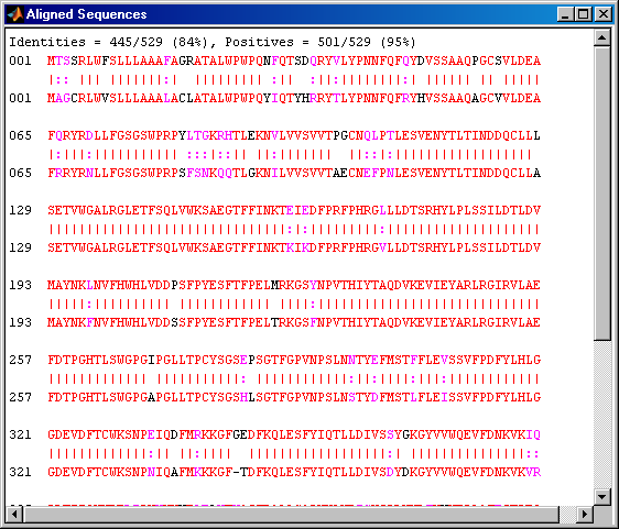
This is still not a perfect alignment at the beginning of the sequence. In order to align the sequences starting with the Met1 we can go back to the information about the ORFs in the nucleotide sequences. Remember that the ORF for the human HEXA gene was on the third reading frame and on the first reading frame for the mouse HEXA gene.
humanPORF = nt2aa(humanHEXA.Sequence(humanORFs(3).Start(1):humanORFs(3).Stop(1)));
mousePORF = nt2aa(mouseHEXA.Sequence(mouseORFs(1).Start(1):mouseORFs(1).Stop(1)));
[score, alignment] = nwalign(humanPORF,mousePORF);
showalignment(alignment);
Alternatively, you can use the coding region information (CDS) from the GenBank data structure to find the coding region of the genes. You can also get the translation of the coding regions from this structure.
humanCodingRegion = humanHEXA.Sequence(...
            humanHEXA.CDS.indices(1):humanHEXA.CDS.indices(2));
mouseCodingRegion = mouseHEXA.Sequence(...
    mouseHEXA.CDS.indices(1):mouseHEXA.CDS.indices(2));

humanTranslatedRegion = humanHEXA.CDS.translation;
mouseTranslatedRegion = mouseHEXA.CDS.translation;
Instead of truncating the sequences to look for better alignment, an alternative approach is to use a local alignment. The function swalign performs local alignment using the Smith-Waterman algorithm. This shows a very good alignment for the whole coding region and reasonable similarity for a few residues beyond at both the ends of the gene.
[score, localAlignment] = swalign(humanProtein,mouseProtein);
showalignment(localAlignment);