BIOGRAPHDEMO Tools for rendering interconnected graph data

Contents

Representing a phylogenetic tree as a graph

Read a phylogenetic tree into a PHYTREE object.

tr = phytreeread('pf00002.tree');

Reduce the tree to only the human proteins (to make the example smaller, you can also use the full tree by omitting the following lines).

sel = getbyname(tr,'human');
tr = prune(tr,~sel(1:37))

    Phylogenetic tree object with 10 leaves (9 branches)

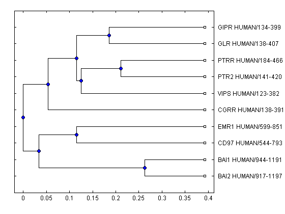
The plot method for a PHYTREE object can create a basic layout of the phylogenetic tree; however, the graph elements are static.

plot(tr)

The PHYTREE object information can be put into a BIOGRAPH object, so you can create a dynamic layout. First, pull some information from the PHYTREE object.

[names,nn,nb,nl] = get(tr,'NodeNames','NumNodes','NumBranches','NumLeaves');
names

names = 

    'BAI2_HUMAN/917-1197'
    'BAI1_HUMAN/944-1191'
    'CD97_HUMAN/544-793'
    'EMR1_HUMAN/599-851'
    'CGRR_HUMAN/138-391'
    'VIPS_HUMAN/123-382'
    'PTR2_HUMAN/141-420'
    'PTRR_HUMAN/184-466'
    'GLR_HUMAN/138-407'
    'GIPR_HUMAN/134-399'
                       ''
                       ''
                       ''
                       ''
                       ''
                       ''
                       ''
                       ''
                       ''

Notice that the names of the branches are empty. This is fine in a PHYTREE object, however, a BIOGRAPH object must have all node IDs unique. Give some arbitrary names to the empty IDs.

for k = nl+1:nn
    names{k} = ['Branch ' num2str(k-nl)];
end

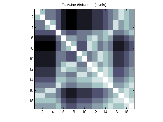
You can build a connection matrix up using the pdist method for the PHYTREE objects. Obtain a pairwise distance matrix by counting tree levels between all possible nodes (leaves and branches). We can visualize this information with the aid of imagesc.

cm = pdist(tr,'criteria','levels','nodes','all','square',true);
figure
imagesc(cm)
colormap(flipud(bone))
axis image
title('Pairwise distances (levels)')

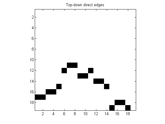
Pick only the entries which are equal to 1 (which indicate that two nodes are directly connected) and entries in the lower triangular part to select top-down direct edges.

cm = tril(cm==1);
figure
imagesc(cm)
colormap(flipud(bone))
axis image
title('Top-down direct edges')

Phylogenetic tree datasets provide the root of the tree as the last element in the set. When building a BIOGRAPH connection matrix, it helps to reverse the order of both the data and names, so that the graph is built from the root out. This will create a more logical and visually appealing presentation.

cm = flipud(fliplr(cm));
names = flipud(names);

Call the BIOGRAPH object constructor with the connection matrix and the node IDs. To explore its properties you can use the get function.

bg = biograph(cm,names)
get(bg)

Biograph object with 19 nodes and 18 edges.
              ID: ''
           Label: ''
     Description: ''
      LayoutType: 'hierarchical'
        EdgeType: 'curved'
           Scale: 1
     LayoutScale: 1
      ShowArrows: 'on'
    NodeAutoSize: 'on'
    NodeCallback: 'display'
    EdgeCallback: 'display'
           Nodes: [19x1 biograph.node]
           Edges: [18x1 biograph.edge]

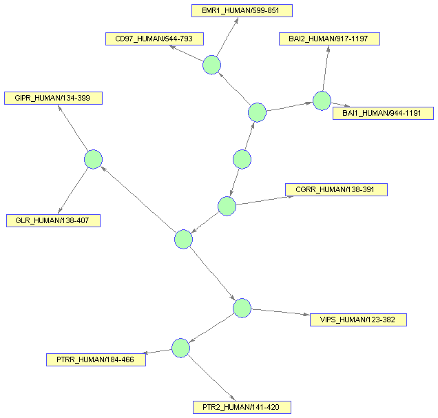
Once a BIOGRAPH object has been created with the essential information (the connection matrix and node IDs), you can modify its properties. For example, change the layout type to 'radial', which is best for phylogenetic data and the scale.

bg.LayoutType = 'radial';
bg.LayoutScale = 3/4;
get(bg)

              ID: ''
           Label: ''
     Description: ''
      LayoutType: 'radial'
        EdgeType: 'curved'
           Scale: 1
     LayoutScale: 0.7500
      ShowArrows: 'on'
    NodeAutoSize: 'on'
    NodeCallback: 'display'
    EdgeCallback: 'display'
           Nodes: [19x1 biograph.node]
           Edges: [18x1 biograph.edge]

Although nodes and edges have been created, the BIOGRAPH object does not have the coordinates in which the graph elements should be drawn such that its rendering results into a pretty and uncluttered display. Before rendering a BIOGRAPH object, you need to calculate an appropriate location for every node. dolayout is the method that calls the layout engine.

Some properties of the BIOGRAPH object interact with the layout engine, among them 'LayoutType' which selects the layout algorithm.

dolayout(bg)

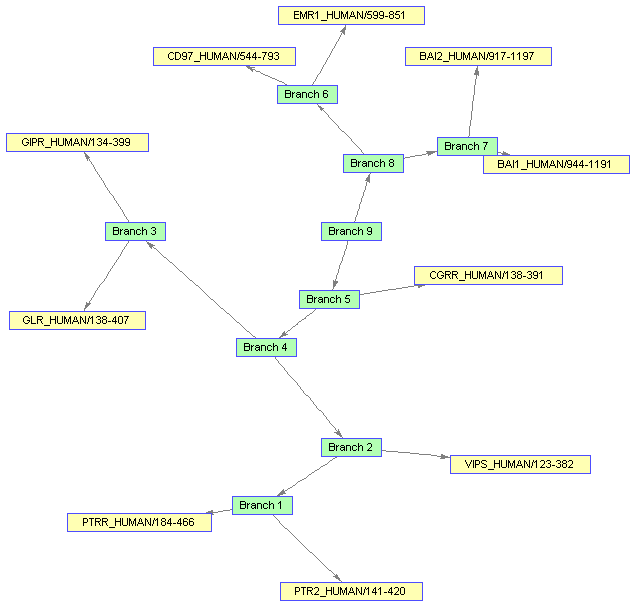
Draw the BIOGRAPH object in a viewer window. The method VIEW creates a Graphical User Interface (GUI) with the interconnected graph and returns a handle to a deep copy of the BIOGRAPH object and which is contained by the figure. With this object handle you can later change some of the rendering properties.

bgInViewer = view(bg)

Biograph object with 19 nodes and 18 edges.

Changing the BIOGRAPH object properties

You might want to change the color of all the nodes that represent branches. Knowing that the first 'nb' nodes are branches, you can use the vectorized form of set to change the 'Color' property of these nodes.

set(bgInViewer.Nodes(1:nb),'Color',[.7 1 .7])

Changing some properties requires you to run the layout engine again. First change the 'Shape' of the branches to circles.

set(bgInViewer.Nodes(1:nb),'Shape','circle')

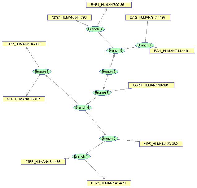
Notice that the new shape is an ellipse and the edges do not connect nicely to the limits of new shapes.

Now, run the layout engine over the BIOGRAPH object contained by the viewer to correct the shapes and the edges.

dolayout(bgInViewer)

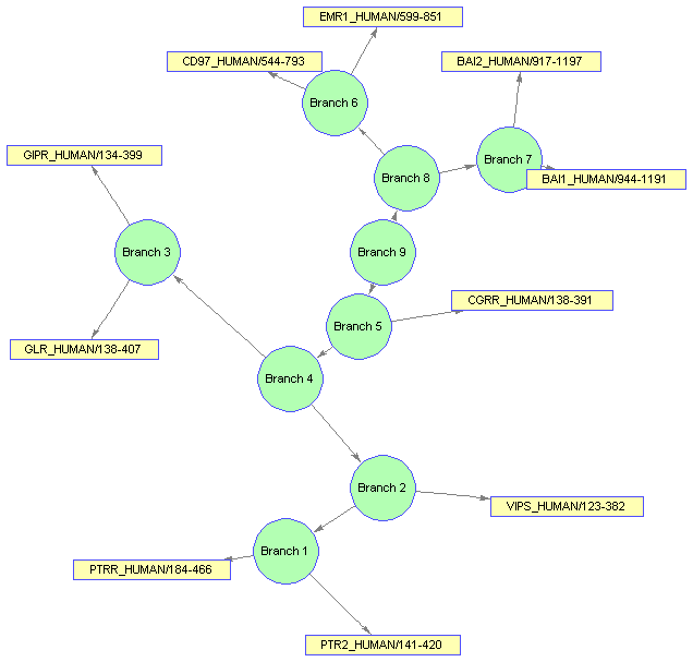
The extent (size) of the nodes is estimated automatically using the node 'FontSize' and 'Label' properties. You can force the nodes to have any size by turning off the BIOGRAPH 'NodeAutoSize' property and then refreshing the layout.

bgInViewer.NodeAutoSize = 'off';
set(bgInViewer.Nodes(1:nb),'Size',[20 20])
set(bgInViewer.Nodes(1:nb),'Label','')
dolayout(bgInViewer)

Copyright 2003-2004 The MathWorks, Inc.
Published with MATLAB® 7.0.2