This example demonstrates a number of ways to classify mass spectrometry data and shows some statistical tools that can be used to look for potential disease markers and proteomic pattern diagnostics.
Serum proteomic pattern diagnostics can be used to differentiate samples from patients with and without disease. Profile patterns are generated using surface-enhanced laser desorption and ionization (SELDI) protein mass spectrometry. This technology has the potential to improve clinical diagnostics tests for cancer pathologies. The goal is to select a reduced set of measurements or "features" that can be used to distinguish between cancer and control patients. These features will be ion intensity levels at specific mass/charge values.
The data in this example is from the FDA-NCI Clinical Proteomics Program Databank (http://home.ccr.cancer.gov/ncifdaproteomics/ppatterns.asp ). This example uses the high-resolution ovarian cancer data set that was generated using the WCX2 protein array. The sample set includes 93 controls and 120 ovarian cancers. An extensive description of this data set and excellent introduction to this promising technology can be found in [1].
This demonstration assumes that you have already downloaded, uncompressed, and preprocessed the raw mass-spectrometry data. You can use msbatchprocessing to preprocess the spectrograms, as explained in biodistcompdemo. (OvarianCancerQAQCdataset.mat is not distributed with MATLAB.)
load OvarianCancerQAQCdataset
whos
  Name      Size                    Bytes  Class

  MZ    15000x1                     60000  single array
  Y     15000x213                12780000  single array

Grand total is 3210000 elements using 12840000 bytes
Initialize some variables that will be used through out the demonstration.
N = 213;                                % Number of samples
lbls = {'Cancer','Normal'};             % Group labels
grp = lbls([ones(120,1);ones(93,1)+1]); % Ground truth
Cidx = strcmp('Cancer',grp);            % Logical index vector for Cancer samples
Nidx = strcmp('Normal',grp);            % Logical index vector for Normal samples
xAxisLabel = 'Mass/Charge (M/Z)';       % x label for plots
yAxisLabel = 'Ion Intensity';           % y label for plots
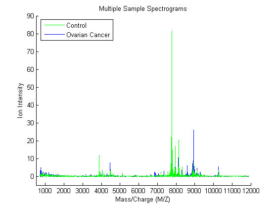
You can plot some data sets into a figure window to visually compare profiles from the two groups; in this example five spectrograms from cancer patients (red) and five from control patients (blue) are displayed.
figure; hold on;
hC = plot(MZ,Y(:,1:5) ,'b');
hN = plot(MZ,Y(:,121:125),'g');
xlabel(xAxisLabel); ylabel(yAxisLabel);
axis([500 12000 -5 90])
legend([hN(1),hC(1)],{'Control','Ovarian Cancer'},2)
title('Multiple Sample Spectrograms')
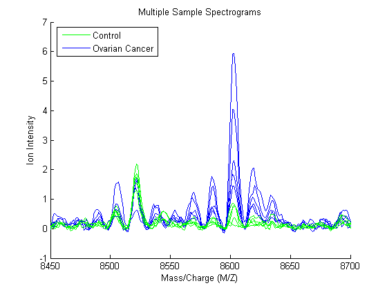
Zooming in on the region from 8500 to 8700 M/Z shows some peaks that might be useful for classifying the data.
axis([8450,8700,-1,7])
Another way to visualize the whole data set is to look at the group average signal for the control and cancer samples. You can plot the group average and the envelopes of each group.
mean_N = mean(Y(:,Nidx),2);  % group average for control samples
max_N = max(Y(:,Nidx),[],2); % top envelopes of the control samples
min_N = min(Y(:,Nidx),[],2); % bottom envelopes of the control samples
mean_C = mean(Y(:,Cidx),2);  % group average for cancer samples
max_C = max(Y(:,Cidx),[],2); % top envelopes of the control samples
min_C = min(Y(:,Cidx),[],2); % bottom envelopes of the control samples

figure; hold on;
hC = plot(MZ,mean_C,'b');
hN = plot(MZ,mean_N,'g');
gC = plot(MZ,[max_C min_C],'b--');
gN = plot(MZ,[max_N min_N],'g--');
xlabel(xAxisLabel);ylabel(yAxisLabel);
axis([8450,8700,-1,7])
legend([hN,hC,gN(1),gC(1)],{'Control Group Avg.','Ovarian Cancer Group Avg',...
                            'Control Envelopes','Ovarian Cancer Envelopes'},2)
title('Group Average and Group Envelopes')
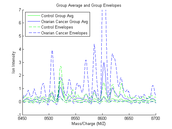
Observe that apparently there is no single feature that can discriminate both groups perfectly.
A naive approach for finding significant features is to assume that each M/Z value is independent and compute a two-way t-test. sqtlfeatures returns an index to the most significant M/Z values, for instance 100 indices ranked by its absolute value of the test statistic.
[feat,stat] = sqtlfeatures(Y,grp,'CRITERION','ttest','NUMBER',100);
The first output of sqtlfeatures (feat indices) can be used to extract the M/Z values of the significant features.
sig_Masses = MZ(feat);
sig_Masses(1:7)' %display the first seven
ans =

  1.0e+003 *

  Columns 1 through 6

    8.1008    8.1018    8.1028    8.0999    8.1038    7.7370

  Column 7

    7.7360
The second output of sqtlfeatures (stat) is a vector with the absolute value of the test statistic. You can plot it over the spectra using plotyy.
figure; hold on;
ax_handle = plotyy(MZ,[mean_N mean_C],MZ,stat);
title('Significant M/Z Values')
axis(ax_handle(1),[7950,8300,-1,20])
legend(ax_handle(1),{'Control Group Avg.','Ovarian Cancer Group Avg.'},2)
xlabel(ax_handle(1),xAxisLabel); ylabel(ax_handle(1),yAxisLabel);
axis(ax_handle(2),[7950,8300,-1,22])
ylabel(ax_handle(2),'Test Statistic');
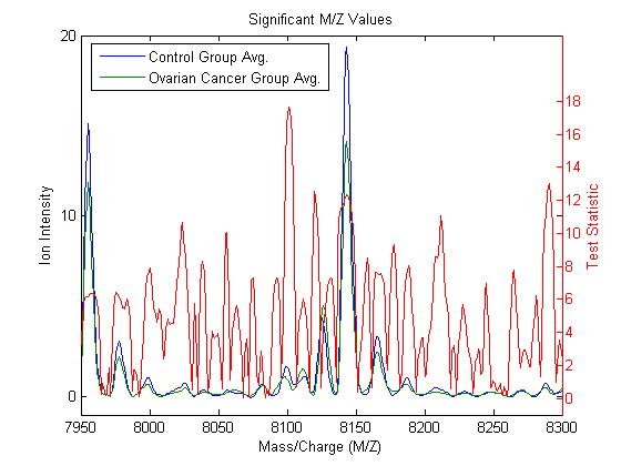
Notice that there are significant regions at high M/Z values but low intensity (~8100 Da.). Other methods to measure class separabilty are available in sqtlfeatures, such as entropy based, Brattacharyya, or the area under the empirical receiver operating characteristic (ROC) curve.
Now that you have identified some significant features, you can use this information to classify the cancer and normal samples. Due to the small number of samples, you can run a cross-validation using the 20% holdout method to have a better estimation of the classifier performance. crossvalind allows you to set the training and test sets for other types of system evaluation methods, such as K-fold and Leave-M-Out.
Observe that features are selected only from the training subset and the validation is performed with the test subset. classperf allows you to keep track of multiple validations.
cp_lda1 = classperf(grp); % initializes the CP object
per_eval = 0.20;          % training size for cross-validation
for k=1:10 % run cross-validation 10 times
    [train,test] = crossvalind('holdout',grp,per_eval);
    feat = sqtlfeatures(Y(:,train),grp(train),'NUMBER',100);
    c = classify(Y(feat,test)',Y(feat,train)',grp(train));
    classperf(cp_lda1,c,test); % updates the CP object with current validation
end
After the loop you can assess the performance of the overall blind classification using any of the properties in the CP object, such as the error rate, sensitivity, specificity, and others.
cp_lda1
                        Label: ''
                  Description: ''
                  ClassLabels: {2x1 cell}
                  GroundTruth: [213x1 double]
         NumberOfObservations: 213
               ControlClasses: 2
                TargetClasses: 1
            ValidationCounter: 10
           SampleDistribution: [213x1 double]
            ErrorDistribution: [213x1 double]
    SampleDistributionByClass: [2x1 double]
     ErrorDistributionByClass: [2x1 double]
               CountingMatrix: [3x2 double]
                  CorrectRate: 0.8405
                    ErrorRate: 0.1595
              LastCorrectRate: 0.8571
                LastErrorRate: 0.1429
             InconclusiveRate: 0
               ClassifiedRate: 1
                  Sensitivity: 0.8208
                  Specificity: 0.8667
      PositivePredictiveValue: 0.8914
      NegativePredictiveValue: 0.7839
           PositiveLikelihood: 6.1563
           NegativeLikelihood: 0.2067
                   Prevalence: 0.5714
              DiagnosticTable: [2x2 double]
This naive approach for feature selection can be improved by eliminating some features based on the regional information. For example, 'NWEIGHT' in sqtlfeatures outweighs the test statistic of neighboring M/Z features such that other significant M/Z values can be incorporated into the subset of selected features
cp_lda2 = classperf(grp); % initializes the CP object
per_eval = 0.20;          % training size for cross-validation
for k=1:10 % run cross-validation 10 times
    [train,test] = crossvalind('holdout',grp,per_eval);
    feat = sqtlfeatures(Y(:,train),grp(train),'NUMBER',100,'NWEIGHT',5);
    c = classify(Y(feat,test)',Y(feat,train)',grp(train));
    classperf(cp_lda2,c,test); % updates the CP object with current validation
end
cp_lda2.CorrectRate % average correct classification rate
ans =

    0.9405
Lilien et al. presented in [2] an algorithm to reduce the data dimensionality that uses principal component analysis (PCA), then LDA is used to classify the groups. In this example 2000 of the most significant features in the M/Z space are mapped to the 150 principal components
cp_pcalda = classperf(grp); % initializes the CP object
per_eval = 0.20;            % Training size for cross-validation
for k=1:10 % run cross-validation 10 times
    [train,test] = crossvalind('holdout',grp,per_eval);
    % select the 2000 most significant features.
    feat = sqtlfeatures(Y(:,train),grp(train),'NUMBER',2000);
    % PCA to reduce dimensionality
    P = princomp(Y(feat,train)','econ');
    % Project into PCA space
    x = Y(feat,:)' * P(:,1:150);
    % Use LDA
    c = classify(x(test,:),x(train,:),grp(train));
    classperf(cp_pcalda,c,test);
end
cp_pcalda.CorrectRate % average correct classification rate
ans =

    0.9881
Feature selection can also be reinforced by classification. Randomized feature selection generates random subsets of features and assesses their quality independently. Later, it selects a pool of the most frequent good features. Li et al. in [3] apply this concept to the analysis of protein expression patterns. randfeatures allows you to search a subset of features using LDA or a k-nearest neighbor classifier over randomized subsets of features.
Note: the following example is computationally intensive, so it has been disabled from the demo. Also, for better results you should increase the pool size and the stringency of the classifier from the default values in randfeatures. Type help randfeatures for more information.
if 0  % <== change to 1 to enable
   [train,test] = crossvalind('holdout',grp,per_eval);
   feat = randfeatures(Y(:,train),grp(train),'CLASSIFIER','da');
else
   load randFeatCancerDetect
end
Assess the quality of the selected feutures with the evaluation set.
P = princomp(Y(feat(1:700),train)','econ');
x = Y(feat(1:700),:)' * P(:,1:10);
c = classify(x(test,:),x(train,:),grp(train));
cp_rndfeat = classperf(grp,c,test);
cp_rndfeat.CorrectRate % average correct classification rate
ans =

     1
There are many classification tools in MATLAB that you can also use to analyze proteomic data. Among them are support vector machines (svmclassify/svmtrain), k-nearest neighbors (knnclassify), neural networks (Neural Network Toolbox), and classification trees (treefit). For feature selection, you can also use a genetic algorithm (Genetic Algorithm and Direct Search (GADS) Toolbox) to optimize this search.
[1] T.P. Conrads, et al., "High-resolution serum proteomic features for ovarian detection", Endocrine-Related Cancer, 11, 2004, pp. 163-178.
[2] R.H. Lilien, et al., "Probabilistic Disease Classification of Expression-Dependent Proteomic Data from Mass Spectrometry of Human Serum", Journal of Computational Biology, 10(6), 2003, pp. 925-946.
[3] L. Li, et al., "Application of the GA/KNN method to SELDI proteomics data", Bioinformatics, 20(10), 2004, pp. 1638-1640.
[4] E.F. Petricoin, et al., "Use of proteomic patterns in serum to identify ovarian cancer", Lancet, 359(9306), 2002, pp. 572-577.