MSPREPRODEMO Preprocessing of raw mass spectrometry data

Contents

Loading the data

Mass spectrometry data is usually stored in text files with two columns, the mass/charge (M/Z) values and the intensity values corresponding to these M/Z ratios. To load the data use one of the following I/O MATLAB functions: importdata, csvread, or textread, or you can use jcampread to load JCAMP-DX formatted files and xlsread to load a spreadsheet in an Excel workbook.

For this demonstration, we use spectrograms taken from one of the low-resolution ovarian cancer NCI/FDA data sets. These spectra were generated using the WCX2 protein-binding chip, two with manual sample handling and two with a robotic sample dispenser/processor

Files are comma separated and start at the second row (after the headers), most of the times importdata can figure out the structure of the data

sample = importdata('mspec01.csv')

sample = 

          data: [15154x2 double]
      textdata: {'M/Z'  'Intensity'}
    colheaders: {'M/Z'  'Intensity'}

The M/Z values are in the first column of the 'data' field and the ion intensities are in the second

MZ = sample.data(:,1);
Y  = sample.data(:,2);

You can also load multiple spectrograms and concatenate them into a single matrix. Now, use csvread instead to load the files. Note: we assume that the M/Z values are the same, for data sets with different M/Z values, use msresample to create a uniform M/Z vector.

files = {'mspec01.csv','mspec02.csv','mspec03.csv','mspec04.csv'};

for i = 1:4
    D = csvread(files{i},1); % starts after the first row
    Y(:,i) = D(:,2);
end

With the plot command you can inspect the loaded spectrograms

plot(MZ,Y)
axis([0 20000 -20 105])
xlabel('Mass/Charge (M/Z)');ylabel('Relative Intensity')
title('Four Low-Resolution Mass Spectrometry Examples')

Resampling the spectra

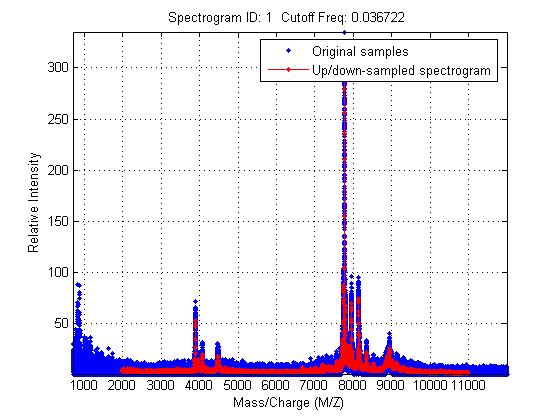
Resampling mass spectrometry data has several advantages: It homogenizes the mass/charge (M/Z) vector, allowing you to compare different spectra under the same reference and at the same resolution. In high-resolution data sets, the large size of the files leads to computationally intensive algorithms. However, high-resolution spectra can be redundant. By resampling one can decimate the signal into a more manageable M/Z vector, preserving the information content of the spectra. msresample allows you to select a new M/Z vector and also applies an antialias filter that prevents high-frequency noise from folding into lower frequencies.

Load a high-resolution spectrum example taken from the high-resolution ovarian cancer NCI/FDA data set. In this case you will use some spectra examples already saved in .mat format.

load sample_hi_res
numel(MZ_hi_res)

ans =

      355760

Down-sample the spectra to 10000 M/Z points between 2000 and 11000. Most of the mass spectrometry preprocessing tools have an input parameter 'SHOWPLOT' that creates a customized plot that helps you to follow and assess the quality of the preprocessing action.

[MZH,YH] = msresample(MZ_hi_res,Y_hi_res,10000,'RANGE',[2000 11000],'SHOWPLOT',true);

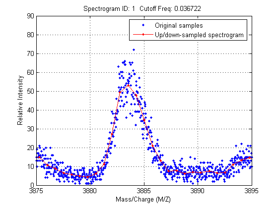
Zooming into a reduced region reveals the detail of the down-sampling procedure.

axis([3875 3895 0 90])

Baseline correction

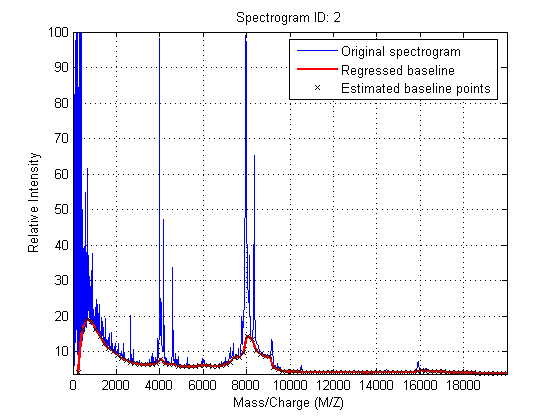
Mass spectrometry data usually shows a varying baseline caused by the chemical noise in the matrix or by ion overloading. msbackadj estimates a low-frequency baseline which is hidden among high-frequency noise and signal peaks. Then the baseline is subtracted from the spectrogram.

To show how to correct the baseline, the demo uses four low-resolution examples, taken from two different NCI/DFA ovarian data sets.

Adjust the baseline of the set of spectrograms and show only the second one and its estimated background.

YB = msbackadj(MZ,Y,'WINDOWSIZE',500,'QUANTILE',0.20,'SHOWPLOT',2);

Aligning a set of spectrograms

Miss-calibration of the mass spectrometer leads to variations of the relation between the observed M/Z vector and the true time of flight of the ions. Therefore, systematic shifts can appear in repeated experiments. When a known profile of peaks is expected in the spectrogram, you can use msalign to standardize the M/Z values.

To align spectrograms you need to provide a set of M/Z values where reference peaks are expected to appear. You can also define a vector with relative weights which is used by the aligning algorithm to emphasize peaks with small area.

P = [3991.4 4598 7964 9160]; % M/Z location of reference peaks
W = [60 100 60 100];         % Weight for reference peaks

Use a heat map to observe the alignment of the spectra before and after applying the alignment algorithm.

msheatmap(MZ,YB,'MARKERS',P,'LIMIT',[3000 10000])
title('Before Alignment')

Align the set of spectrograms to the reference peaks given.

YA = msalign(MZ,YB,P,'WEIGHTS',W);

msheatmap(MZ,YA,'markers',P,'limit',[3000 10000])
title('After Alignment')

Normalization

In repeated experiments, it is also common to find systematic differences in the total amount of desorbed and ionized proteins. To compensate for this, the relative intensities of the spectrograms are normalized (or standardized).

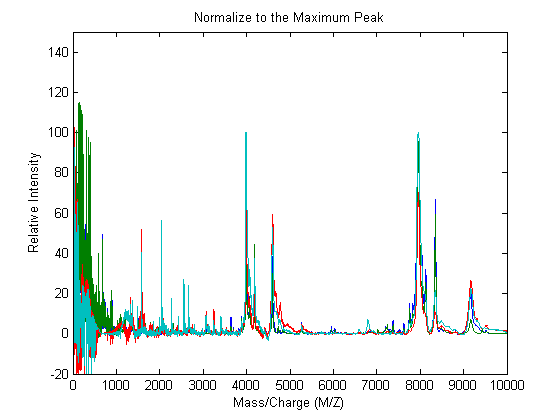
One of many methods to standardize the values of the spectrograms is to rescale the maximum intensity of every signal to a certain value, for instance 100. It is also possible to ignore problematic regions; for example, in serum samples you might want to ignore the low-mass region (M/Z < 1000 Da.).

YN1 = msnorm(MZ,YA,'QUANTILE',1,'LIMITS',[1000 inf],'MAX',100);
plot(MZ,YN1)
axis([0 10000 -20 150])
xlabel('Mass/Charge (M/Z)');ylabel('Relative Intensity')
title('Normalize to the Maximum Peak')

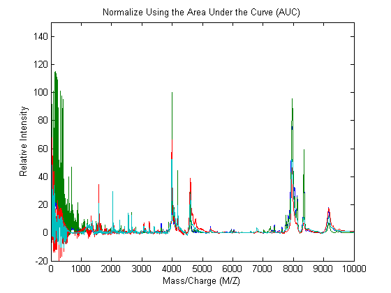
msnorm can also standardize using the area under the curve (AUC) and then rescale the spectrograms to have relative intensities below 100.

YN2 = msnorm(MZ,YA,'LIMITS',[1000 inf],'MAX',100);
plot(MZ,YN2)
axis([0 10000 -20 150])
xlabel('Mass/Charge (M/Z)');ylabel('Relative Intensity')
title('Normalize Using the Area Under the Curve (AUC)')

Noise reduction

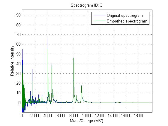
Standardized spectra usually contains a mixture of noise and signal. Some applications require you to denoise the spectrograms in order to improve the validity and precision of the observed mass/charge values of the peaks in the spectra. For the same reason, denoising also improves further peak detection algorithms. However, it is important to preserve as much as possible the sharpness (or high-frequency components) of the peak. For this, you can use Lowess smoothing and polynomial filters.

Smooth the spectrograms with a polynomial filter of second order.

 YS = mssgolay(MZ,YN2,'SPAN',35,'SHOWPLOT',3);

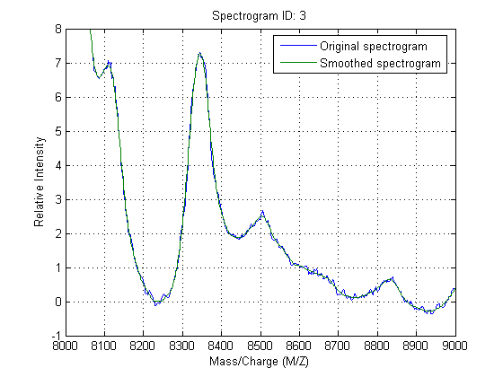
Zooming into a reduced region reveals the detail of the smoothing algorithm.

axis([8000 9000 -1 8])

Peak finding

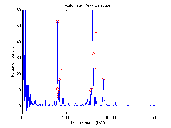
A naive approach to find putative peaks is to look at the first derivative of the smoothed signal, then some of these locations can be filtered to avoid small ion-intensity peaks and low-mass peaks.

slopeSign = diff(YS(:,1))>0;
slopeSignChange = diff(slopeSign)<0;
h = find(slopeSignChange) + 1; % finds all peaks

h(MZ(h) < 1500) = [];   % eliminate peaks in the low-mass region

h(YS(h,1) < 5) = [];           % eliminate small peaks

plot(MZ,YS(:,1),'-',MZ(h),YS(h,1),'ro')
axis([0 15000 -5 60])
xlabel('Mass/Charge (M/Z)');ylabel('Relative Intensity')
title('Automatic Peak Selection')

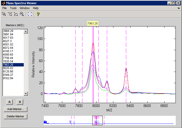
Use msviewer to inspect some of the preprocessed spectrograms.

msviewer(MZ,YS,'MARKERS',MZ(h),'GROUP',1:4)

Copyright 2003-2004 The MathWorks, Inc.
Published with MATLAB® 7.0.1