This demonstration looks at some statistics about the DNA content of the human mitochondrial genome.
Mitochondria are generally the major energy production center in eukaryotes. The Genome repository at the NCBI contains more interesting information about the human mitochondrial genome.
web('http://www.ncbi.nlm.nih.gov/genomes/framik.cgi?db=Genome&gi=12188')
The consensus sequence of the human mitochondria genome has accession number NC_001807. The whole GenBank entry is quite large and this example only uses the nucleotide sequence, so you can use the getgenbank function with the 'SequenceOnly' flag to read just the sequence information into the MATLAB workspace.
mitochondria = getgenbank('NC_001807','SequenceOnly',true);
If you don't have a live web connection, you can load the data from a MAT-file using the command
% load mitochondria % <== Uncomment this if no internet connection
The MATLAB whos command gives information about the size of the sequence.
whos mitochondria
  Name               Size                    Bytes  Class

  mitochondria       1x16571                 33142  char array

Grand total is 16571 elements using 33142 bytes
You will use some of the sequence statistics function in the Bioinformatics Toolbox to look at various properties of this sequence. You can look at the composition of the nucleotides with the ntdensity function.
ntdensity(mitochondria)
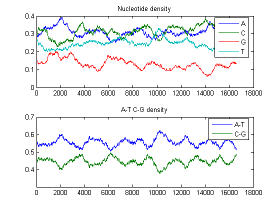
This shows that the genome is A-T rich. You can get more specific information with the basecount function.
basecount(mitochondria)
ans =
    A: 5113
    C: 5192
    G: 2180
    T: 4086
These are on the 5'-3' strand. You can look at the reverse complement using the seqrcomplement function.
basecount(seqrcomplement(mitochondria))
ans =
    A: 4086
    C: 2180
    G: 5192
    T: 5113
As expected, the base counts on the reverse complement strand are complementary to the counts on the 5'-3' strand.
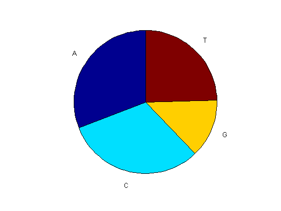
You can use the chart option to basecount to display a pie chart of the distribution of the bases.
figure
basecount(mitochondria,'chart','pie');
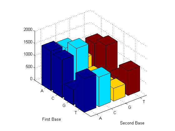
Now look at the dimers in the sequence and display the information in a bar chart using dimercount.
figure
dimercount(mitochondria,'chart','bar')
ans =
    AA: 1594
    AC: 1495
    AG: 801
    AT: 1223
    CA: 1536
    CC: 1779
    CG: 439
    CT: 1438
    GA: 615
    GC: 716
    GG: 427
    GT: 421
    TA: 1368
    TC: 1202
    TG: 512
    TT: 1004
You can look at codons using codoncount. The function dimercount simply counts all adjacent nucleotides; however codoncount counts the codons on a particular reading frame. With no options, the function shows the codon counts on the first reading frame.
codoncount(mitochondria)
AAA - 172     AAC - 157     AAG -  67     AAT - 123
ACA - 153     ACC - 163     ACG -  42     ACT - 130
AGA -  58     AGC -  90     AGG -  50     AGT -  43
ATA - 132     ATC - 103     ATG -  57     ATT -  96
CAA - 166     CAC - 167     CAG -  68     CAT - 135
CCA - 146     CCC - 215     CCG -  50     CCT - 182
CGA -  33     CGC -  60     CGG -  18     CGT -  20
CTA - 187     CTC - 126     CTG -  52     CTT -  98
GAA -  68     GAC -  62     GAG -  47     GAT -  39
GCA -  67     GCC -  87     GCG -  23     GCT -  61
GGA -  53     GGC -  61     GGG -  23     GGT -  25
GTA -  61     GTC -  49     GTG -  26     GTT -  36
TAA - 136     TAC - 127     TAG -  82     TAT - 107
TCA - 143     TCC - 126     TCG -  37     TCT - 103
TGA -  64     TGC -  35     TGG -  27     TGT -  25
TTA - 115     TTC - 113     TTG -  37     TTT -  99
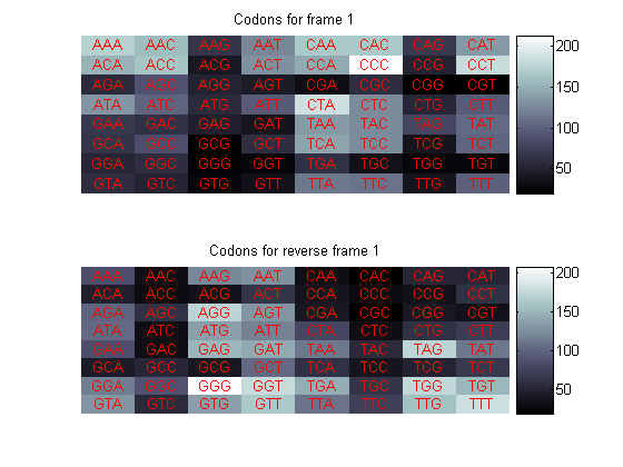
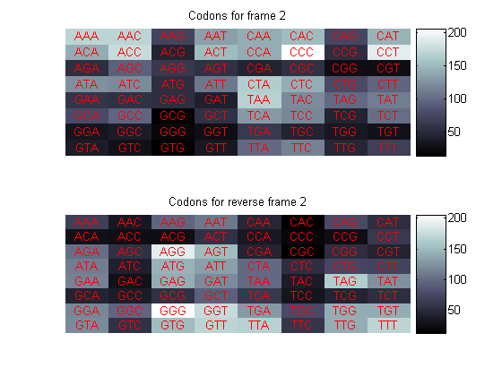
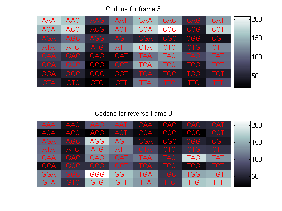
Using a loop you can also look at all the other reading frames:
for frame = 1:3
    figure
    subplot(2,1,1); codoncount(mitochondria,'frame',frame,'figure',true);
    title(sprintf('Codons for frame %d',frame));
    subplot(2,1,2); codoncount(mitochondria,'reverse',true,'frame',frame,'figure',true);
    title(sprintf('Codons for reverse frame %d',frame));
end
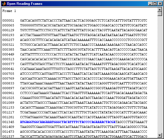
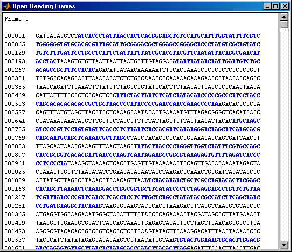
In a nucleotide sequence an obvious thing to look for is if there are any open reading frames. The function seqshoworfs can be used to visualize ORFs in a sequence. Note: In the HTML tutorial only the first page of the output is shown, however when running the demo you will be able to inspect the complete mitochondrial genome using the scrollbar on the figure.
seqshoworfs(mitochondria);
If you compare this output to the genes shown on the NCBI page there seem to be slightly fewer ORFs, and hence fewer genes, than expected. Vertebrate mitochondria do not use the Standard genetic code so some codons have different meaning in mitochondrial genomes. For more information about using different genetic codes in MATLAB see the help for the function geneticcode.
help geneticcode
 GENETICCODE returns a structure containing mappings for the genetic code.

    MAP = GENETICCODE returns a structure containing mapping for the Standard
    genetic code.

    GENETICCODE(ID) returns a structure of the mapping for alternate genetic
    codes, where ID is either the transl_table ID from the NCBI Genetics web
    page (http://www.ncbi.nlm.nih.gov/Taxonomy/Utils/wprintgc.cgi?mode=c)
    or one of the following supported names. NAME can be truncated to the
    first two characters of the name.

    ID  Name

  	1	Standard
  	2	Vertebrate Mitochondrial
  	3	Yeast Mitochondrial
  	4	Mold, Protozoan, and Coelenterate Mitochondrial and Mycoplasma/Spiroplasma
  	5	Invertebrate Mitochondrial
  	6	Ciliate, Dasycladacean and Hexamita Nuclear
  	9	Echinoderm Mitochondrial
  	10	Euplotid Nuclear
  	11	Bacterial and Plant Plastid
  	12	Alternative Yeast Nuclear
  	13	Ascidian Mitochondrial
  	14	Flatworm Mitochondrial
  	15	Blepharisma Nuclear
  	16	Chlorophycean Mitochondrial
  	21	Trematode Mitochondrial
  	22	Scenedesmus Obliquus Mitochondrial
  	23	Thraustochytrium Mitochondrial

    Examples:

        moldcode = geneticcode(4)
        wormcode = geneticcode('Flatworm Mitochondrial')

    See also <a href="matlab:help aa2nt">aa2nt</a>, <a href="matlab:help aminolookup">aminolookup</a>, <a href="matlab:help baselookup">baselookup</a>, <a href="matlab:help nt2aa">nt2aa</a>, <a href="matlab:help revgeneticcode">revgeneticcode</a>, <a href="matlab:help seqshoworfs">seqshoworfs</a>.


    Reference page in Help browser
       <a href="matlab:doc geneticcode">doc geneticcode</a>
The 'GeneticCode' option to the seqshoworfs function allows you to look at the ORFs again but this time with the vertebrate mitochondrial genetic code. Notice that there are now two much larger ORFs on the first reading frame: One starting at position 4471 and the other starting at 5905. These correspond to the ND2 (NADH dehydrogenase subunit 2) and COX1 (cytochrome c oxidase subunit I) genes.
orfs = seqshoworfs(mitochondria,'GeneticCode','Vertebrate Mitochondrial',...
        'alternativestart',true)
orfs =
1x3 struct array with fields:
    Start
    Stop
The ORF of interest starts at position 4471, the following commands can be used to find the corresponding stop codon:
ND2Start = 4471;
startIndex = find(orfs(1).Start == ND2Start)
ND2Stop = orfs(1).Stop(startIndex)
startIndex =
    24
ND2Stop =
        5512
Once the positions are known, MATLAB indexing can be used to extract the region of interest.
ND2Seq = mitochondria(ND2Start:ND2Stop);
If you look at the codoncount for this gene we see a lot of CTA and ATC codons.
codoncount(ND2Seq)
AAA - 10     AAC - 14     AAG -  2     AAT -  6
ACA - 11     ACC - 24     ACG -  3     ACT -  5
AGA -  0     AGC -  4     AGG -  0     AGT -  1
ATA - 22     ATC - 24     ATG -  2     ATT -  8
CAA -  8     CAC -  3     CAG -  2     CAT -  1
CCA -  4     CCC - 12     CCG -  2     CCT -  5
CGA -  0     CGC -  3     CGG -  0     CGT -  1
CTA - 26     CTC - 18     CTG -  4     CTT -  7
GAA -  5     GAC -  0     GAG -  1     GAT -  0
GCA -  8     GCC -  7     GCG -  1     GCT -  4
GGA -  5     GGC -  7     GGG -  0     GGT -  1
GTA -  3     GTC -  2     GTG -  0     GTT -  3
TAA -  0     TAC -  8     TAG -  0     TAT -  2
TCA -  7     TCC - 11     TCG -  1     TCT -  4
TGA - 10     TGC -  0     TGG -  1     TGT -  0
TTA -  8     TTC -  7     TTG -  1     TTT -  8
For those of you who have not memorized the genetic code you can easily check what amino acids these codons get translated into using the nt2aa and aminolookup functions.
aminolookup('code',nt2aa('CTA'))
aminolookup('code',nt2aa('ATC'))
ans =
Leu	Leucine

ans =
Ile	Isoleucine
The nt2aa function converts the nucleotide sequence to the corresponding amino acid sequence. Again the 'GeneticCode' option must be used to specify the vertebrate mitochondrial genetic code.
ND2 = nt2aa(ND2Seq,'GeneticCode','Vertebrate Mitochondria');
You can get a more complete picture of the amino acid content with aacount.
figure
aacount(ND2,'chart','bar')
ans =
    A: 20
    R: 4
    N: 20
    D: 0
    C: 0
    Q: 10
    E: 6
    G: 13
    H: 4
    I: 31
    L: 64
    K: 12
    M: 25
    F: 15
    P: 23
    S: 28
    T: 43
    W: 11
    Y: 10
    V: 8
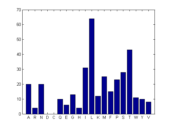
Notice the high leucine, threonine and isoleucine content and also the lack of cysteine or aspartic acid.
You can use the atomiccomp and molweight functions to find out more about the ND2 protein.
atomiccomp(ND2)
molweight(ND2)
ans =
    C: 1818
    H: 2882
    N: 420
    O: 471
    S: 25
ans =
  3.8960e+004
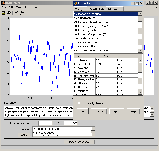
For further investigation of the properties of the ND2 protein, try using proteinplot. This is a graphical user interface (GUI) that allows you to easily create plots of various properties, such as hydrophobicity, of a protein sequence. Click on the "Help" menu in the GUI for more information on how to use the tool.
proteinplot(ND2)