The Control System Toolbox provides commands for creating 4 basic types of linear time-invariant (LTI) models:
These functions take model data as input and return objects which embody this data in a single MATLAB variable.
where:


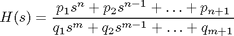
The numerator and denominator polynomials define a transfer function model.
A vector of coefficients specifies the polynomials. For example
[ 1, 2, 10 ]
would specify the polynomial

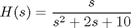
You can create a SISO transfer function model by specifying its numerator and denominator polynomials as inputs to the TF command:
num = [ 1  0 ];       % Numerator: s
den = [ 1  2  10 ];   % Denominator: s^2 + 2 s + 10
H = tf(num,den);
You can also specify this model as a rational expression of s:
s = tf('s');        % Create Laplace variable
H = s / (s^2 + 2*s + 10);
where


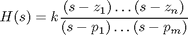
Zero-pole-gain models are the factored form of transfer function models.
In this format, the gain k, zeros z (numerator roots), and poles p (denominator roots) characterize the model.
You can specify a SISO zero-pole-gain model using the ZPK command:
z = 0;                   % Zeros
p = [ 2  1+i  1-i ];     % Poles
k = -2;                  % Gain
H = zpk(z,p,k);
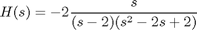
You can also specify this model as a rational expression of s:
s = zpk('s');
H = -2*s / (s - 2) / (s^2 - 2*s + 2);


where


State-space models are constructed from the linear differential or difference equations describing the system dynamics.
The state-space matrices A, B, C, and D characterize these models.
The following describes a simple electric motor.
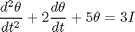
where


The relations below describe the relationship between the driving current (input) and the angular displacement of the rotor (output) in state-space form.


%
% You can use the SS command to create the state-space model of this system
% in MATLAB:

A = [ 0  1 ; -5  -2 ];
B = [ 0 ; 3 ];
C = [ 1  0 ];
D = 0;
H = ss(A,B,C,D);
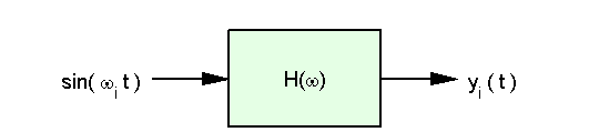
Frequency response data, FRD, models allow you to store the measured or simulated complex frequency response of a system in an LTI object. You can then analyze the model using the Control System Toolbox.
Given a vector of frequencies and a vector of system responses to excitation at these frequencies,
From input 1 to:
        Frequency(Hz)      output 1
        -------------      --------
             1000      -0.8126-0.0003i
             2000      -0.1751-0.0016i
             3000      -0.0926-0.4630i
you can construct an FRD model with this data using the FRD command:
freq = [1000 ; 2000 ; 3000];  % measured in Hz
resp = [-0.8126-0.0003i ; -0.1751-0.0016i ; -0.0926-0.4630i];
H = frd(resp,freq,'Units','Hz');
The last 2 arguments in this example are used to indicate that the frequency units are in Hertz. The MATLAB output is shown above.