Mixing disparate time scales or unit scales can produce state-space models with coefficients that are widely spread in value. Working with such poorly scaled models can lead to numerical instabilities and puzzling results.
Below is an example of a poorly-scaled model (POORBAL). Note the many orders of magnitude separating the entries of B and C, as well as the lower vs. upper diagonal entries in the state matrix A:
load numdemo            % load POORBAL model
format short g
[a,b,c,d] = ssdata(poorbal)
a =

      -4275.4   -0.0037741     0.017311    -0.066733
 -2.6809e+009        -2900       -14966 -1.7386e+006
 -5.8087e+008       706.98 -1.0015e+006  3.8709e+006
  1.4051e+008       5153.2  2.4289e+005 -9.3906e+005


b =

 -1.0307e+015
  1.7073e+021
 -1.7231e+021
  4.1797e+020


c =

 -1.3095e-008  3.0534e-014  6.5238e-013 -2.5219e-012


d =

       1122.9
This model is stable with poles at: -1.9e6, -2.6e3+7.0e4i, -2.6e3-7.0e4i, -4.3e3
To illustrate the problems of poor scaling, discretize the model at 1 MHz (Ts = 1e-6) using the matrix-based version of C2D, and then simulate the step response:
clf;
ax = gca;
axis(ax,'normal')
[ad,bd] = c2d(a,b,1e-6);
step(ss(ad,bd,c,d,1e-6),1e-3);
title('Step Response of discretized POORBAL (unbalanced)')
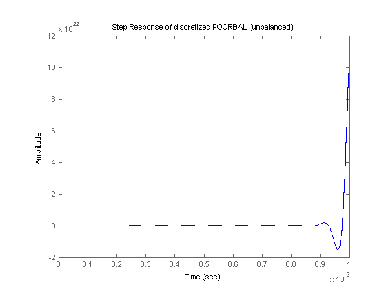
The response diverges in spite of the continuous-time model being stable. The C2D conversion fails to preserve stability on this badly-scaled model.
A useful command to remedy poor scaling is SSBAL. This command takes a state-space model and rescales the states to compress the range of numerical values in the A,B,C matrices. This operation is called "balancing":
wellbal = ssbal(poorbal);
[a,b,c,d] = ssdata(wellbal)
a =

      -4275.4      -3957.4         4538      -4373.4
      -2556.7        -2900      -3741.5 -1.0866e+005
      -2215.8       2827.9 -1.0015e+006  9.6773e+005
         2144        82451  9.7156e+005 -9.3906e+005


b =

      -3749.7
       5923.4
       -23913
        23202


c =

      -3599.5       8800.8        47009       -45431


d =

       1122.9
The balanced model is shown above. Note the significantly reduced spread in numerical values.
Next, repeat the same discretization and simulation steps with the balanced model (WELLBAL):
[ad,bd] = c2d(a,b,1e-6);
step(ss(ad,bd,c,d,1e-6),1e-3)
title('Step Response of discretized WELLBAL (balanced)');
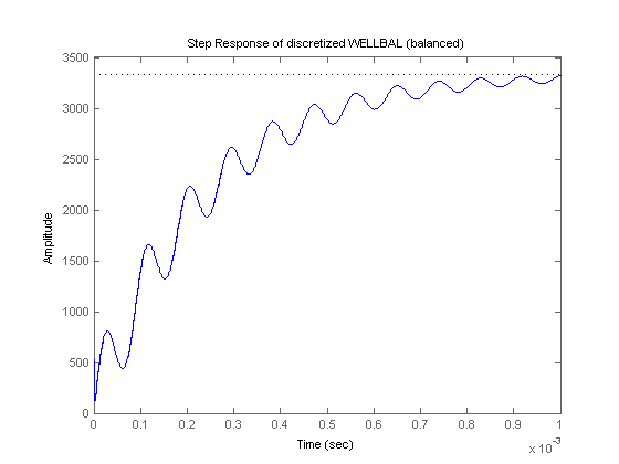
The simulation now produces the expected results.
Many commands in the Control System Toolbox perform balancing automatically. This includes C2D when applied to a state-space model (as opposed to A,B matrices):
poorbal_d = c2d(poorbal,1e-6);
step(poorbal_d,1e-3)
title('Step Response of POORBAL\_D (balanced)');
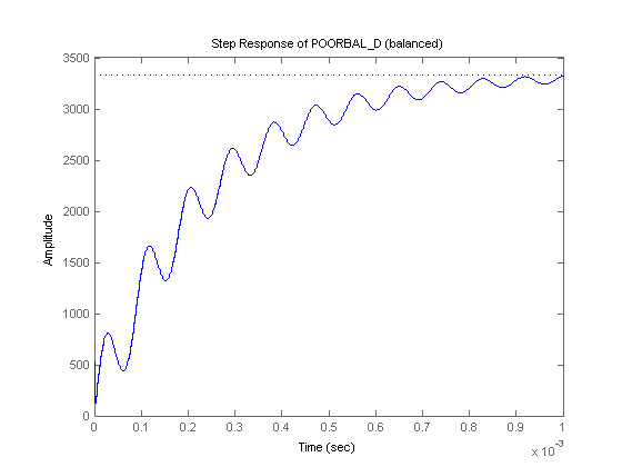
Note that the discretized model is now stable thanks to the balancing performed by C2D behind the scenes.
Moral: Avoid working with poorly scaled models and use SSBAL to correct scaling problems.