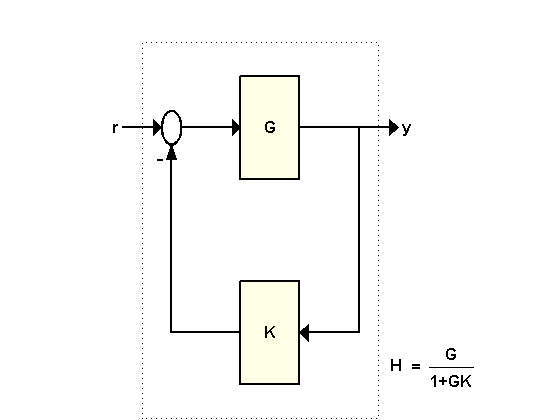
For the feedback loop shown above with
G = tf([1 2],[1 .5 3]);
K = 2;
the best way to compute the closed-loop transfer function H from r to y is to use the FEEDBACK command:
H = feedback(G,K)
Transfer function:
     s + 2
---------------
s^2 + 2.5 s + 7
From the formula H = G/(1+GK), you could also consider computing H directly as
H2 = G/(1+G*K)
Transfer function:
      s^3 + 2.5 s^2 + 4 s + 6
-----------------------------------
s^4 + 3 s^3 + 11.25 s^2 + 11 s + 21
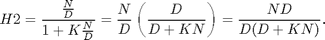
Unfortunately, the second approach gives bad results in general, as shown above. This is because the expression H2, with G = N/D, is evaluated generically as
Therefore the poles of G are added to both the numerator and denominator of H.
This can have dramatic consequences when computing with high-order transfer functions. The more sophisticated example below involves a 17th order transfer function G. Compute the closed-loop transfer function for K=1
load numdemo                 % load G model

H1 = feedback(G,1);          % good

H2 = G/(1+G);                % bad
and compare the closed-loop Bode plots:
ax = gca;
axis(ax,'auto')
bode(H1,'b',H2,'r')
title('H1 (blue) vs. H2 (red)');
h = gcr;
set(h.AxesGrid,'XUnits','rad/sec','YUnits',{'dB';'deg'});
ax = getaxes(h.AxesGrid);
set(ax(1),'Ylim',[-50 0]);
set(ax(2),'Ylim',[-360 360]);
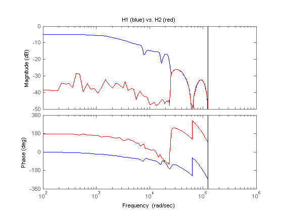
The errors in the low frequency response of H2 can be traced to the additional (cancelling) dynamics introduced near z=1. Specifically, H2 has about twice as many poles and zeros near z=1 than H1. As a result, the values of H2 near z=1 have poor accuracy which distorts the response at low frequencies. See the "High-Order Transfer Functions" topic for more details.
Moral: Always use the FEEDBACK command to close feedback loops.