You can connect LTI models using +, *, [ , ], [ ; ], and the commands SERIES, PARALLEL, and FEEDBACK. To ensure that the resulting model has minimal order, it is important to follow some simple rules:
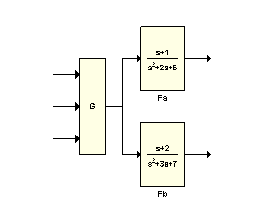
As an example, try to compute a model for the block diagram sketched above, with
G = [1 , tf(1,[1 0]) , 5];
Fa = tf([1 1] , [1 2 5]);
Fb = tf([1 2] , [1 3 7]);
Let's start with the "optimal" way to connect these three blocks:
H1 = [ss(Fa) ; ss(Fb)] * G;
Note that (a) Fa and Fb are converted to state space, and (b) this operation mirrors the block diagram structure. The resulting model H1 has order 5, which is minimal:
size(H1,'order')
ans =

     5
Let's now look at the "worst" way to derive a state-space model for this block diagram. Observing that the overall transfer function is H = [Fa * G ; Fb * G], you could compute H as
H2 = ss( [Fa * G ; Fb * G] );
size(H2,'order')
ans =

    14
The order of the resulting model H2 is 14, almost three times higher than H1!
While H2 is a valid model, it contains a lot of duplicated dynamics because (a) G appears twice in the expression, and (b) the state-space conversion is performed on a 2x3 MIMO transfer matrix.
Here are a couple additional combinations with their respective fortunes:
H3 = ss( [Fa ; Fb] * G );      % order = 14
H4 = ss( [Fa ; Fb] ) * G;      % order = 5, lucky...
Moral: Use the state-space form for model interconnections, and stay true to the block diagram structure.