Poles of high multiplicity and clusters of nearby poles can be very sensitive to round off errors, sometimes with dramatic consequences. This example compares the response of a 15th-order discrete-time state-space model, Hss, with that of its equivalent transfer function model, Htf:
load numdemo               % load Hss model
Htf = tf(Hss);
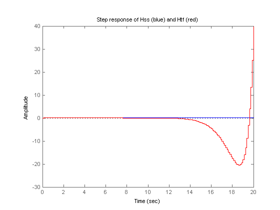
The step response of Htf diverges even though the state-space model, Hss, is stable (all poles lie in the unit circle):
ax = gca;
axis(ax,'normal')
step(Hss,'b',Htf,'r',20)
title('Step response of Hss (blue) and Htf (red)');
A comparison of the Bode plots is not any more favorable:
bode(Hss,'b',Htf,'r')
h = gcr;
title('Bode diagram of Hss (blue) and Htf (red)');
set(h.AxesGrid,'XUnits','rad/sec','YUnits',{'dB';'deg'});
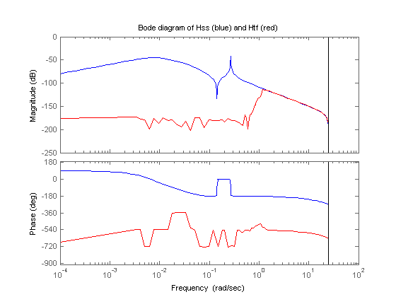
Again, the transfer function''s response is quite erratic.
To understand these large discrepancies compare the pole/zero maps of the state-space model and its transfer function:
pzmap(Hss,'b',Htf,'r')
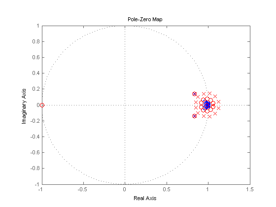
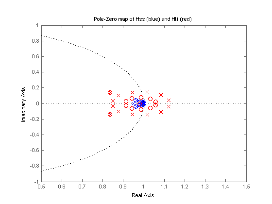
Note the tighly packed cluster of poles near z=1 in Hss. When these poles are recombined into the transfer function denominator, roundoff errors perturb the pole cluster into an evenly-distributed ring of poles around z=1 (a typical pattern for perturbed multiple roots). Unfortunately here, some perturbed poles cross the unit circle, making the transfer function unstable:
pzmap(Hss,'b',Htf,'r');
h = gcr;
title('Pole-Zero map of Hss (blue) and Htf (red)');
h.AxesGrid.setxlim([0.5 1.5]);
h.AxesGrid.setylim([-1.0 1.0]);
h.FrequencyUnits = 'rad/sec';

pa = getaxes(h.AxesGrid);
t = 0:.01:2*pi;
line('Parent',double(pa),'XData',cos(t),'YData',sin(t),'color','k','linestyle',':')
A simple experiment confirms these explanations:
pss = pole(Hss);                   % poles of Hss
Den = poly(pss);                   % polynomial with roots Pss
ptf = roots(Den);                  % roots of this polynomial
plot(real(pss),imag(pss),'bx',real(ptf),imag(ptf),'r*')
title('Poles of Hss (blue) vs. roots of Den (red)');
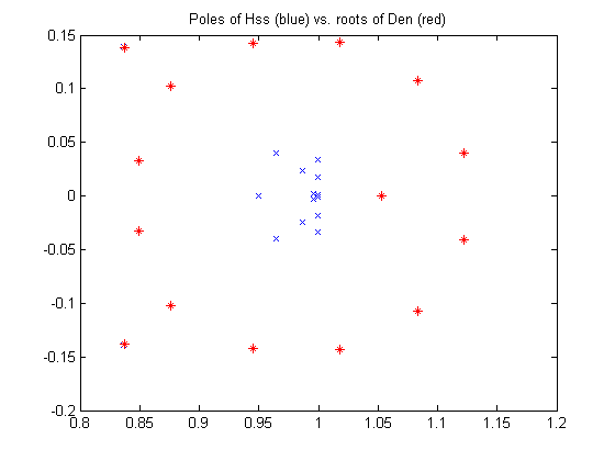
This shows that ROOTS(POLY(R)) can be quite different from R for clustered roots.
Moral: Beware of poles or zeros of high multiplicity.