This gallery illustrates the range of maps that you can create using geoshow.
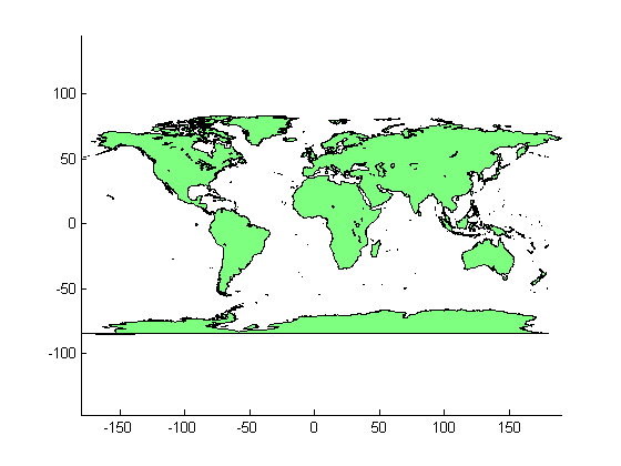
Display world land areas, without a projection.
figure
geoshow('landareas.shp', 'FaceColor', [0.5 1.0 0.5]);
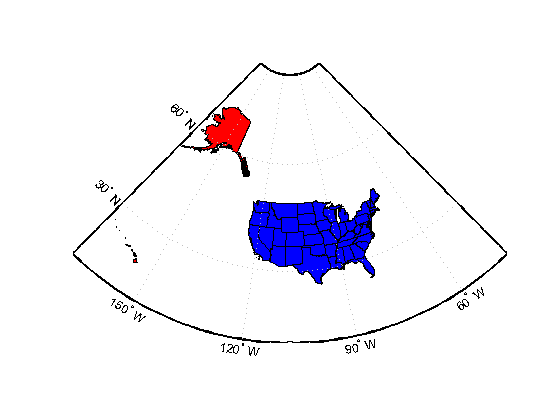
Read the USA high resolution data.
states = shaperead('usastatehi', 'UseGeoCoords', true);
Create a SymbolSpec to display Alaska and Hawaii as red polygons.
symbols = makesymbolspec('Polygon', ...
                        {'Name', 'Alaska', 'FaceColor', 'red'}, ...
                        {'Name', 'Hawaii', 'FaceColor', 'red'});
Create a worldmap of North America with Alaska and Hawaii in red, all other states in blue.
figure
worldmap('na');
geoshow(states, 'SymbolSpec', symbols, ...
               'DefaultFaceColor', 'blue', ...
               'DefaultEdgeColor', 'black');
axis off
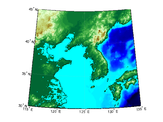
Load the Korean data grid and the land area boundary.
load korea
S = shaperead('landareas','UseGeoCoords',true);
Create a worldmap and display the Korean data grid as a texture map.
figure;
worldmap(map, refvec)
geoshow(gca, map, refvec, 'DisplayType', 'texturemap');
colormap(demcmap(map))
axis off

Overlay the land area boundary as a line.
geoshow([S.Lat], [S.Lon]);
Load the geoid data.
load geoid
Create an Eckert projection axes and display the geoid as a texture map.
figure
axesm eckert4; framem; gridm;
h = geoshow(geoid, geoidrefvec, 'DisplayType','texturemap');
axis off
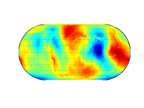
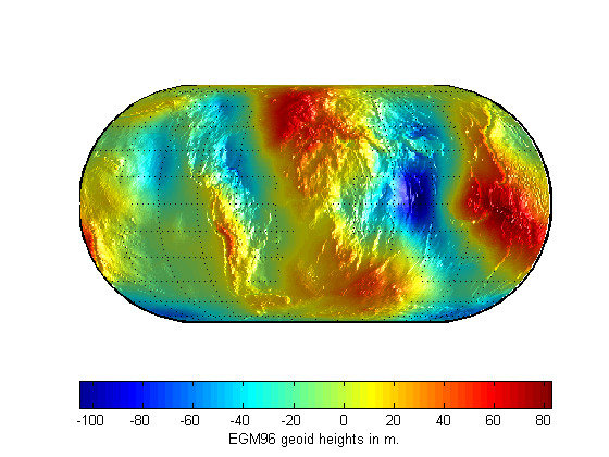
Set the Z data to the geoid height values, rather than a surface with zero elevation.
set(h,'ZData',geoid);
light;
material(0.6*[1 1 1]);

set(gca,'dataaspectratio',[1 1 200]);
hcb = colorbar('horiz');
set(get(hcb,'Xlabel'),'String','EGM96 geoid heights in m.')
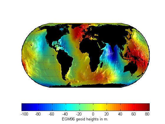
Mask out all the land.
geoshow('landareas.shp', 'FaceColor', 'black');
zdatam(handlem('patch'), max(geoid(:)));
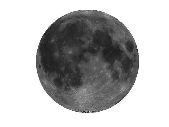
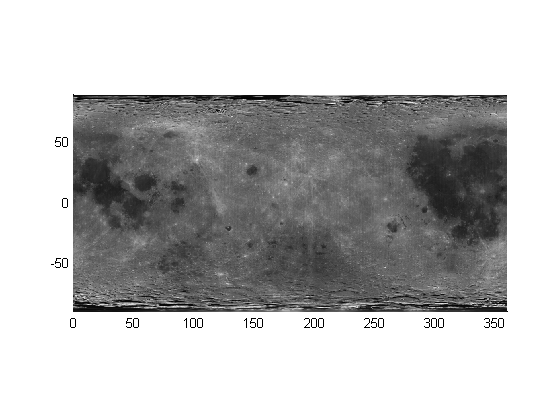
Load the moon albedo image.
load moonalb
Display the moon albedo image unprojected.
figure
geoshow(moonalb,moonalbrefvec)
Display the moon albedo image in an orthographic projection.
figure
axesm ortho
geoshow(moonalb, moonalbrefvec)
axis off