Differential Equations in MATLAB

Contents

Initial value problem

VANDERPOLDEMO is a function that defines the van der Pol equation.

type vanderpoldemo

function dydt = vanderpoldemo(t,y,Mu)
%VANDERPOLDEMO Defines the van der Pol equation for ODEDEMO.

% Copyright 1984-2002 The MathWorks, Inc.  
% $Revision: 1.2 $  $Date: 2002/06/17 13:20:38 $ 

dydt = [y(2); Mu*(1-y(1)^2)*y(2)-y(1)];

The equation is written as a system of two first order ODEs. These are evaluated for different values of the parameter Mu. For faster integration, we choose an appropriate solver based on the value of the parameter Mu.

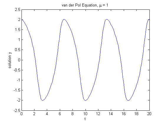
For Mu = 1, any of the MATLAB ODE solvers can solve the van der Pol equation efficiently. The ODE45 solver used below is one such example. The equation is solved in the domain [0, 20].

tspan = [0, 20];
y0 = [2; 0];
Mu = 1;
[t,y] = ode45(@vanderpoldemo, tspan, y0,[],Mu);

% Plot of the solution
plot(t,y(:,1))
xlabel('t')
ylabel('solution y')
title('van der Pol Equation, \mu = 1')

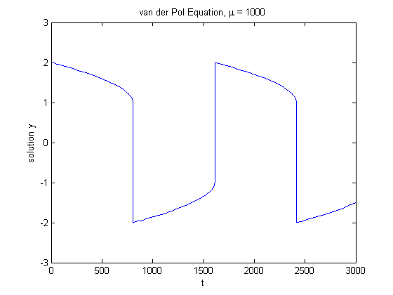
For larger magnitudes of Mu, the problem becomes stiff. Special numerical methods are needed for fast integration. ODE15S, ODE23S, ODE23T, and ODE23TB can solve stiff problems efficiently.

Here is a solution using ODE15S to solve the van der Pol equation for Mu = 1000.

tspan = [0, 3000];
y0 = [2; 0];
Mu = 1000;
[t,y] = ode15s(@vanderpoldemo, tspan, y0,[],Mu);

plot(t,y(:,1))
title('van der Pol Equation, \mu = 1000')
axis([0 3000 -3 3])
xlabel('t')
ylabel('solution y')

Boundary value problems

The function TWOODE has a differential equation written as a system of two first order ODEs.

type twoode

function dydx = twoode(x,y)
%TWOODE  Evaluate the differential equations for TWOBVP. 
% 
%   See also TWOBC, TWOBVP. 

%   Lawrence F. Shampine and Jacek Kierzenka
%   Copyright 1984-2002 The MathWorks, Inc.  
%   $Revision: 1.5 $  $Date: 2002/04/15 03:37:29 $ 

dydx = [ y(2); -abs(y(1)) ];

TWOBC has the boundary conditions for TWOODE.

type twobc

function res = twobc(ya,yb)
%TWOBC  Evaluate the residual in the boundary conditions for TWOBVP. 
% 
%   See also TWOODE, TWOBVP. 

%   Lawrence F. Shampine and Jacek Kierzenka
%   Copyright 1984-2002 The MathWorks, Inc.  
%   $Revision: 1.5 $  $Date: 2002/04/15 03:37:33 $ 

res = [ ya(1); yb(1) + 2 ];

We have to provide a guess for the solution we want represented as a mesh. The solver then adapts the mesh as it refines the guess to a possible solution.

BVPINIT forms the initial guess that BVP4C, one of the solvers, will need. For a mesh of [0 1 2 3 4] and a constant guess of y(x) = 1, y'(x) = 0, call it like this:

solinit = bvpinit([0 1 2 3 4],[1; 0]);

With this initial guess, we can solve the problem with BVP4C.

The solution sol (below) is then evaluated at points xint using DEVAL and plotted.

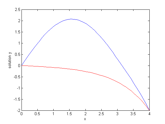
sol = bvp4c(@twoode, @twobc, solinit);

xint = linspace(0, 4, 50);
yint = deval(sol, xint);
plot(xint, yint(1,:),'b');
xlabel('x')
ylabel('solution y')
hold on

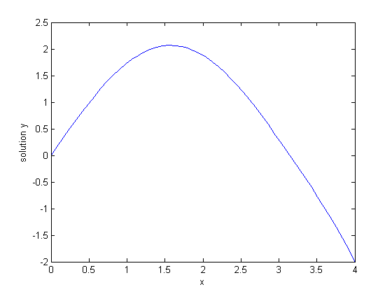
This particular boundary value problem has exactly two solutions. The other solution is obtained for an initial guess of

   y(x) = -1, y'(x) = 0

and plotted as before.

solinit = bvpinit([0 1 2 3 4],[-1; 0]);
sol = bvp4c(@twoode,@twobc,solinit);

xint = linspace(0,4,50);
yint = deval(sol,xint);
plot(xint,yint(1,:),'r');
hold off

Partial differential equations

PDEPE solves partial differential equations in one space variable and time.

The examples PDEX1, PDEX2, PDEX3, PDEX4, PDEX5 form a mini-tutorial on using PDEPE. Browse through these function for more examples.

This example problem uses functions PDEX1PDE, PDEX1IC, and PDEX1BC.

PDEX1PDE defines the differential equation.

type pdex1pde

function [c,f,s] = pdex1pde(x,t,u,DuDx)
%PDEX1PDE  Evaluate the differential equations components for the PDEX1 problem.
%
%   See also PDEPE, PDEX1.

%   Lawrence F. Shampine and Jacek Kierzenka
%   Copyright 1984-2002 The MathWorks, Inc. 
%   $Revision: 1.5 $  $Date: 2002/04/15 03:37:37 $

c = pi^2;
f = DuDx;
s = 0;

PDEX1IC sets up the initial conditions.

type pdex1ic

function u0 = pdex1ic(x)
%PDEX1IC  Evaluate the initial conditions for the problem coded in PDEX1.
%
%   See also PDEPE, PDEX1.

%   Lawrence F. Shampine and Jacek Kierzenka
%   Copyright 1984-2002 The MathWorks, Inc. 
%   $Revision: 1.5 $  $Date: 2002/04/15 03:37:41 $

u0 = sin(pi*x);

PDEX1BC sets up the boundary conditions.

type pdex1bc

function [pl,ql,pr,qr] = pdex1bc(xl,ul,xr,ur,t)
%PDEX1BC  Evaluate the boundary conditions for the problem coded in PDEX1.
%
%   See also PDEPE, PDEX1.

%   Lawrence F. Shampine and Jacek Kierzenka
%   Copyright 1984-2002 The MathWorks, Inc. 
%   $Revision: 1.5 $  $Date: 2002/04/15 03:37:45 $

pl = ul;
ql = 0;
pr = pi * exp(-t);
qr = 1;

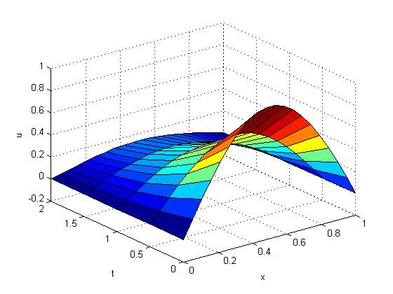
PDEPE requires x, the spatial discretization, and t, a vector of times at which you want a snapshot of the solution. We solve this problem using a mesh of 20 nodes and request the solution at five values of t. Finally, we extract and plot the first component of the solution.

x = linspace(0,1,20);
t = [0 0.5 1 1.5 2];
sol = pdepe(0,@pdex1pde,@pdex1ic,@pdex1bc,x,t);
u1 = sol(:,:,1);
surf(x,t,u1);
xlabel('x');ylabel('t');zlabel('u');
hold on

u1 = sol(:,:,1);

surf(x,t,u1);
xlabel('x'); ylabel('t'); zlabel('u');

Copyright 1984-2002 The MathWorks, Inc.
Published with MATLAB® 7.0.4