This demo describes convex hulls, Delaunay tessellations, and Voronoi diagrams in 3 dimensions. It also shows how to interpolate three-dimensional scattered data.
Many applications in science, engineering, statistics, and mathematics use structures like convex hulls, Delaunay tessellations and Voronoi diagrams for analyzing data. MATLAB enables you to geometrically analyze data sets in any dimension.
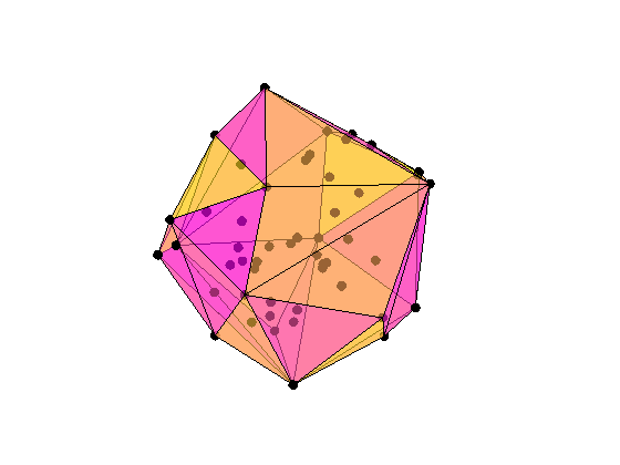
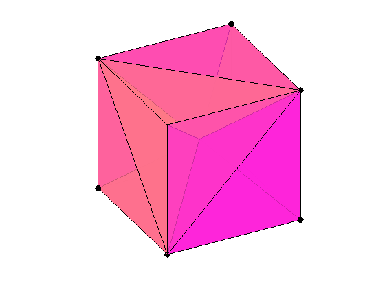
Here, in 3 dimensions, we show a set of 50 points with its convex hull.
% Create the data.
n = 50;
X = randn(n,3);
% Plot the points.
plot3(X(:,1),X(:,2),X(:,3),'ko','markerfacecolor','k');
% Compute the convex hull.
C = convhulln(X);
% Plot the convex hull.
hold on
for i = 1:size(C,1)
   j = C(i,[1 2 3 1]);
   patch(X(j,1),X(j,2),X(j,3),rand,'FaceAlpha',0.6);
end
% Modify the view.
view(3), axis equal off tight vis3d; camzoom(1.2)
colormap(spring)
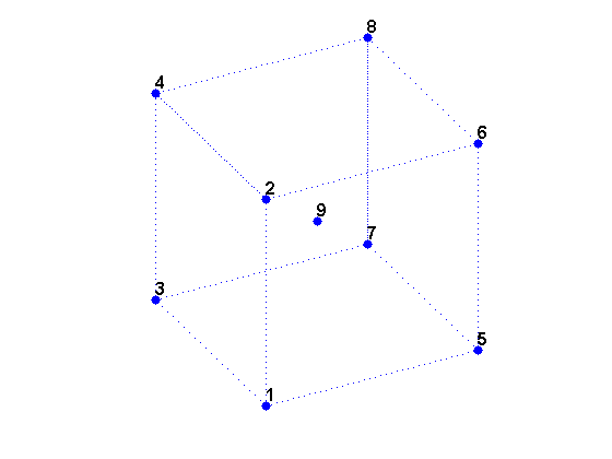
We can create a data set X of the 8 vertices of a cube plus its center.
X is a 9-by-3 matrix where each row is the 3-D coordinates of one point.
% Create X.
X = zeros(8,3);
X([5:8,11,12,15,16,18,20,22,24]) = 1; % Corners.
X(9,:) = [0.5 0.5 0.5]; % Center.
% Visualize X.
cla reset; hold on
d = [1 2 4 3 1 5 6 8 7 5 6 2 4 8 7 3];
plot3(X(d,1),X(d,2),X(d,3),'b:');
plot3(X(:,1),X(:,2),X(:,3),'b.','markersize',20);
t = text(X(:,1),X(:,2),X(:,3), num2str((1:9)'));
set(t,'VerticalAlignment','bottom','FontWeight','bold', 'FontSize',12);
view(3); axis equal tight off vis3d; camorbit(10,0);
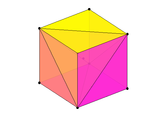
The convex hull of a data set is the smallest convex region that contains the data set. The convex hull of the cube data set X can be computed by CONVHULLN.
For this data set X, the convex hull has 12 facets, each corresponding to a row in K and plotted above with X. The cube is transparent so that you can see all the facets and data points.
% Compute the convex hull.
tri = convhulln(X);
% Plot the data
cla reset;
plot3(X(:,1),X(:,2),X(:,3),'ko','markerfacecolor','k');
% Plot the convex hull.
for i = 1:size(tri,1)
  c = tri(i,[1 2 3 1]);
  patch(X(c,1),X(c,2),X(c,3),i,'FaceAlpha', 0.9);
end
% Modify the view.
view(3); axis equal tight off vis3d
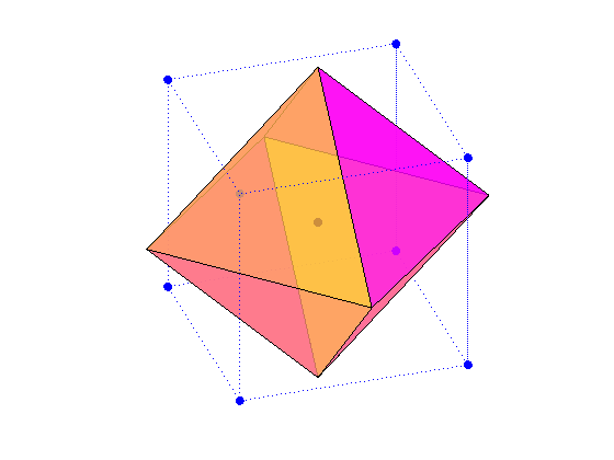
A Delaunay tessellation in 3 dimensions is a set of tetrahedrons such that no data points are contained in any tetrahedron's circumsphere. The Delaunay tessellation of the data set X can be computed by DELAUNAYN.
The 12 rows of T represent the 12 tetrahedrons that partition the data set X.
% Compute the delaunay tessellation.
tri = delaunayn(X);
% Plot the data.
plot3(X(:,1),X(:,2),X(:,3),'ko','markerfacecolor','k');
% Plot the tessellation.
for i = 1:size(tri,1)
  y = tri(i,[1 1 1 2; 2 2 3 3; 3 4 4 4]);
  x1 = reshape(X(y,1),3,4);
  x2 = reshape(X(y,2),3,4);
  x3 = reshape(X(y,3),3,4);
  patch(x1,x2,x3,(1:4)*i,'FaceAlpha',0.8);
end
% Modify the view.
view(3); axis equal tight off vis3d; camorbit(10,0)
A Voronoi diagram partitions the data space into polyhedral regions, with one region for each data point. Anywhere within a region is closer to its data point than any other in the set. The Voronoi diagram of the cube data set X can be computed by VORONOIN.
V is the set of Voronoi vertices. C represents the set of Voronoi regions. For our data set X, C has 9 Voronoi regions. Here we show one Voronoi region, the region for the center point of the cube.
% Compute Voronoi diagram.
[c,v] = voronoin(X);
% Plot the data.
plot3(X(d,1),X(d,2),X(d,3),'b:.',X(9,1),X(9,2),X(9,3),'k.','markersize',20);
% Plot the Voronoi diagram.
nx = c(v{9},:);
tri = convhulln(nx);
for i = 1:size(tri,1)
   patch(nx(tri(i,:),1),nx(tri(i,:),2),nx(tri(i,:),3),rand,'FaceAlpha',0.8);
end
% Modify the view.
view(3); axis equal tight off vis3d; camzoom(1.5); camorbit(20,0)
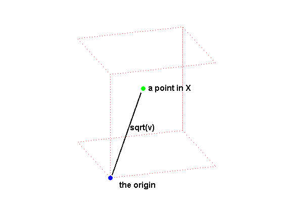
GRIDDATAN interpolates multidimensional scattered data. It uses DELAUNAYN to tessellate the data, and then interpolates based on the tessellation. We start with a data set of 500 random points in 3 dimensions and compute the values of a function, the squared distance from the origin, at each of these points.
% Create the data.
n = 500;
X = 2*rand(n,3)-1;
v = sum(X.^2,2);
% Draw a picture to show how X is defined.
cla reset; hold on
plot3([0.02, 0.47],[0.02,0.57],[0.02,0.57],'k-','linewidth',2);
plot3(0,0,0,'bo','markerfacecolor','b');
cube = zeros(8,3);
cube([5:8,11,12,15,16,18,20,22,24]) = 1; % Corners
cube(9,:) = [0.5 0.5 0.5]; % Center.
plot3(cube(d,1),cube(d,2),cube(d,3),'r:');
plot3(0.5,0.6,0.6,'go','markerfacecolor','g');
text(0.02,-0.2,0,'the origin','fontsize',12,'fontweight','bold');
text(0.55,0.6,0.6,'a point in X','fontsize',12,'fontweight','bold');
text(0.28,0.3,0.35,'sqrt(v)','fontsize',12,'fontweight','bold');
view(3); axis equal tight off vis3d;
camorbit(20,-10);
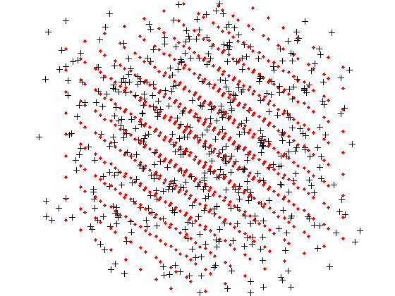
With GRIDDATAN we can interpolate X and the values v over a grid X0 to get the function values v0 over this grid.
The black points are X and the red points are the grid X0.
% Grid the data.
d  = -0.8:0.2:0.8;
[x0,y0,z0] = meshgrid(d,d,d);
X0 = [x0(:) y0(:) z0(:)];
v0 = reshape(griddatan(X,v,X0),size(x0));
% Plot results.
cla reset; hold on;
plot3(X(:,1),X(:,2),X(:,3),'k+','markerfacecolor','k');
plot3(X0(:,1),X0(:,2),X0(:,3),'r.','markerfacecolor','r');
view(3); axis equal tight off vis3d; camzoom(1.6);
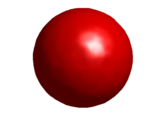
To visualize the surface at all points where the function takes on a constant value, we can use ISOSURFACE and ISONORMALS. Since the function is the squared distance from the origin, the surface at a constant value is a sphere.
c = 0.6;  % constant value
cla reset; hold on;
h = patch(isosurface(x0,y0,z0,v0,c),'FaceColor','red','EdgeColor','none');
isonormals(x0,y0,z0,v0,h);
view(3); axis equal tight off vis3d; camzoom(1.6); camlight; lighting phong
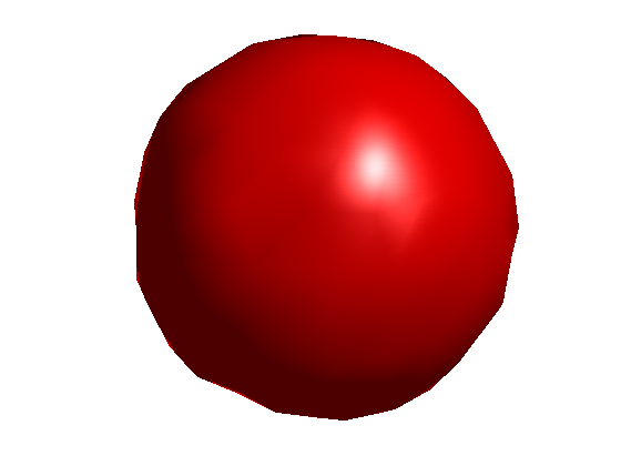
With more data points in X and a denser grid X0, the sphere is smoother but takes longer to compute.
Here is a precomputed sphere generated using 5000 data points in X and a distance between gridpoints of 0.05.
% Load saved results.
load qhulldemo
cla reset; hold on
d = -0.8:0.05:0.8;
[x0,y0,z0] = meshgrid(d,d,d);
h = patch(isosurface(x0,y0,z0,v0,0.6));
isonormals(x0,y0,z0,v0,h);
set(h,'FaceColor','red','EdgeColor','none');
view(3); axis equal tight off vis3d; camzoom(1.6)
camlight; lighting phong