Robustness of Servo Controller for DC Motor

This example demonstrates the data structures for uncertainty modeling, the robustness analysis tools, and the model reduction commands.

Data Structures for Uncertainty Modeling
DC Motor Example
Uncertain Model of DC Motor
Open-loop Analysis
Closed-loop Robustness Analysis
Robustness of Disturbance Rejection Characteristics

Data Structures for Uncertainty Modeling

The Robust Control Toolbox lets you create uncertain elements (e.g., physical parameters whose value is not known exactly) and combine these elements into uncertain models. You can then easily analyze the impact of uncertainty on the control system performance.

For example, consider a plant model

where gamma can range in the interval [3,5] and tau has average value 0.5 with 30% variability. You can create an uncertain model of P(s) by

gamma = ureal('gamma',4,'range',[3 5]);
tau = ureal('tau',.5,'Percentage',30);
P = tf(gamma,[tau 1])

USS: 1 State, 1 Output, 1 Input, Continuous System
  gamma: real, nominal = 4, range = [3  5], 1 occurrence             
    tau: real, nominal = 0.5, variability = [-30  30]%, 2 occurrences

Suppose you have designed an integral controller C for the nominal plant (gamma=4 and tau=0.5). To find out how variations of gamma and tau affect the plant and the closed-loop performance, form the closed-loop system CLP from C and P.

KI = 1/(2*tau.Nominal*gamma.Nominal);
C = tf(KI,[1 0]);
CLP = feedback(P*C,1)

USS: 2 States, 1 Output, 1 Input, Continuous System
  gamma: real, nominal = 4, range = [3  5], 1 occurrence             
    tau: real, nominal = 0.5, variability = [-30  30]%, 2 occurrences

You can now generate 20 random samples of the uncertain parameters gamma and tau and plot the corresponding step responses of the plant and closed-loop models.

subplot(2,1,1); step(usample(P,20)), title('Plant response (20 samples)')
subplot(2,1,2); step(usample(CLP,20)), title('Closed-loop response (20 samples)')

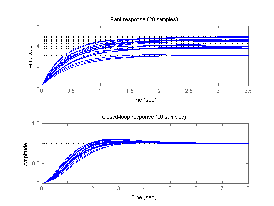
The bottom plot shows that your controller is reasonably robust in spite of significant fluctuations in the plant DC gain.

DC Motor Example

This example builds on the Controls System Toolbox DC motor example by adding parameter uncertainty and unmodeled dynamics and investigating the robustness of the servo controller to such uncertainty.

The nominal model of the DC motor is defined by the resistance R, the inductance L, the emf constant Kb, armature constant Km, the linear approximation of viscous friction Kf and the inertial load J. Each of these components vary within a specific range of values. The resistance and inductance constants range within +/- 40% of their nominal values. The command ureal is used to construct these uncertain parameters.

R = ureal('R',2,'Percentage',40);
L = ureal('L',0.5,'Percentage',40);

The values of Kf and Kb are the same and are correlated. They have a nominal value of 0.015 and range between 0.012 and 0.019 with a nominal value of 0.015. These values are named K.

K = ureal('K',0.015,'Range',[0.012 0.019]);
Km = K;
Kb = K;

Viscous friction, Kf, has a nominal value of 0.2 with a 50% variation in its value.

Kf = ureal('Kf',0.2,'Percentage',50);

The inertia J is also uncertain. It is modeled as a constant 0.02, which is a simplistic model that neglects dynamics present in the real system. We assume that the maximum I/O gain of these dynamics does not exceed 10% of J's nominal value 0.02. These unmodeled dynamics are included in the problem using a ultidyn object.

J = 0.02*(1 + 0.1*ultidyn('Jlti',[1 1],'Bound',1));

Uncertain Model of DC Motor

The differential equations describing the motor dynamics can be written in state-space form as

where

are the current, angular velocity, and applied voltage, respectively.

The uncertain state-space matrices A, B and known matrices C, D are constructed from the motor parameters:

% Create uncertain matrices A,B
A = [1/L 0;0 1/J]*[-R -Kb;Km -Kf];
B = [1/L ; 0];

% Create matrices C,D
C = [0 1];
D = 0;

Note that A and B are uncertain matrix (umat) objects. You then create the uncertain model of the DC motor from these uncertain matrices.

P = ss(A,B,C,D,'StateName',{'Voltage';'Speed'});

For analysis purposes, we use the nominal controller synthesized for the DC motor in the 'Getting Started with the Control System Toolbox' manual

Cont = tf(84*[.233 1],[.0357 1 0]);

Open-loop Analysis

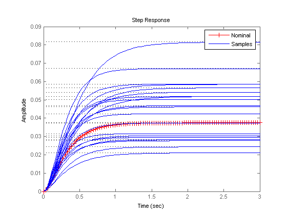
First, compare the step response of the nominal DC motor with 20 samples of the uncertain model of the DC motor.

clf
step(P.NominalValue,'r-+',usample(P,20),'b',3)
legend('Nominal','Samples')

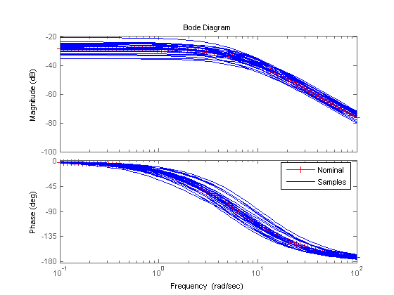
Similarly, you can compare the Bode plot of the open-loop nominal (red) and sampled (blue) uncertain models of the DC motor.

om = logspace(-1,2,80);
Pg = frd(P,om)
bode(Pg.NominalValue,'r-+',usample(Pg,25),'b');
legend('Nominal','Samples')

UFRD: 1 Output, 1 Input, Continuous System, 80 Frequency points
  Jlti: 1x1 LTI, max. gain = 1, 1 occurrence                        
     K: real, nominal = 0.015, range = [0.012  0.019], 2 occurrences
    Kf: real, nominal = 0.2, variability = [-50  50]%, 1 occurrence 
     L: real, nominal = 0.5, variability = [-40  40]%, 1 occurrence 
     R: real, nominal = 2, variability = [-40  40]%, 1 occurrence

Closed-loop Robustness Analysis

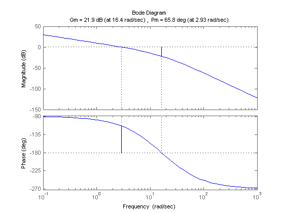
The objective of this section is to analyze the stability and performance robustness of the closed-loop DC motor system. The initial analysis of the nominal closed-loop system indicates the nominal closed-loop system is very robust with 21.8 dB gain margin and 65.8 deg of phase margin.

margin(P.NominalValue*Cont)

The loopmargin command provides comprehensive stability analysis for multivariable feedback systems. For a control system with N feedback channels, loopmargin returns:

The classical gain and phase margins SM for each individual feedback channel (loop-at-a-time margins)
The disk margins DM for each individual feedback channel. The disk margin for the j-th feedback channel indicates by how much the transfer function Lj(s) can vary before this particular loop goes unstable.
The multi-loop disk margin MM, which indicates how much simultaneous, independent gain and phase variations can be tolerated in each feedback channel before the overall closed-loop system goes unstable (same as DM for single-loop control systems).

The guaranteed bounds for DM and MM are calculated based on a balanced sensitivity function.

[SM,DM,MM] = loopmargin(P.NominalValue*Cont);

Classical stability margins

SM

SM = 
     GainMargin: 12.4154
    GMFrequency: 16.4229
    PhaseMargin: 65.7794
    PMFrequency: 2.9349
    DelayMargin: 0.3912
    DMFrequency: 2.9349
         Stable: 1

Disk margin

DM

DM = 
     GainMargin: [0.2790 3.5837]
    PhaseMargin: [-58.8175 58.8175]
      Frequency: 4.9047

Recall that the DC motor plant is uncertain. In addition to the standard gain and phase margins, the worst-case gain/phase margins for the plant-controller feedback loop can be determined using the wcmargin command. wcmargin calculates the worst-case disk gain and phase margins for each input/output channel. The worst-case analysis shows a degradation of the classical gain and phase margins, which were 21.8 dB and 65.8 deg respectively, to a mere 1.5 dB and 10.0 degs.

wcmarg = wcmargin(Pg,Cont)

wcmarg = 
     GainMargin: [0.8388 1.1921]
    PhaseMargin: [-10.0175 10.0175]
      Frequency: 5.1152
    Sensitivity: [1x1 struct]

Robustness of Disturbance Rejection Characteristics

The sensitivity function is a standard measure of closed-loop performance for the feedback system. Compute the uncertain sensitivity function S and compare the Bode magnitude plots for the nominal and sampled uncertain sensitivity function.

S = feedback(1,P*Cont);
bodemag(S.Nominal,'r-+',usample(S,20),'b');
legend('Nominal','Samples')

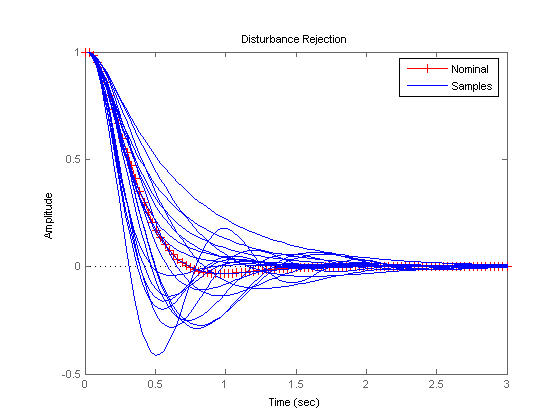
In the time domain, the sensitivity function indicates how well a step disturbance can be rejected. Sample the uncertain sensitivity function and plot its step response to see the variability in disturbance rejection characteristics (nominal appears in red).

step(S.Nominal,'r-+',usample(S,20),'b',3);
title('Disturbance Rejection')
legend('Nominal','Samples')

You can compute the worst-case value of the uncertain sensitivity function gain (peak across frequency) with the wcgain command. Alternatively, you could also use the wcsens command to compute this value.

Sg = frd(S,om);
[maxgain,worstuncertainty] = wcgain(Sg);
maxgain

maxgain = 
           LowerBound: 5.9090
           UpperBound: 5.9946
    CriticalFrequency: 5.1152

With usubs you can substitute the worst-case values of the uncertainty worstuncertainty into the uncertain sensitivity function S. This gives the worst-case sensitivity function Sworst over the entire uncertainty range. Note that the peak gain of Sworst matches with the lower-bound computed by wcgain.

Sworst = usubs(S,worstuncertainty);
Sgworst = frd(Sworst,Sg.Frequency);
norm(Sgworst,inf)
maxgain.LowerBound

ans =
    5.9090
ans =
    5.9090

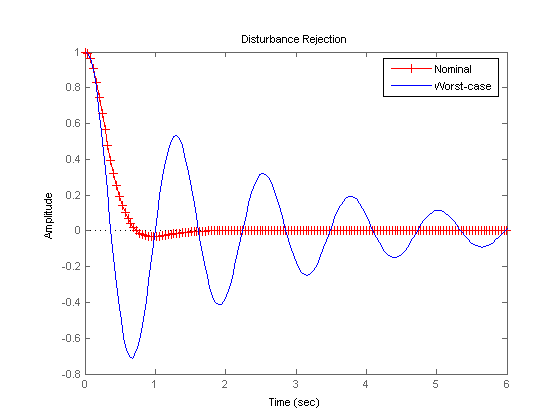
Compare the step responses of the nominal and worst-case sensitivity.

step(S.NominalValue,'r-+',Sworst,'b',6);
title('Disturbance Rejection')
legend('Nominal','Worst-case')

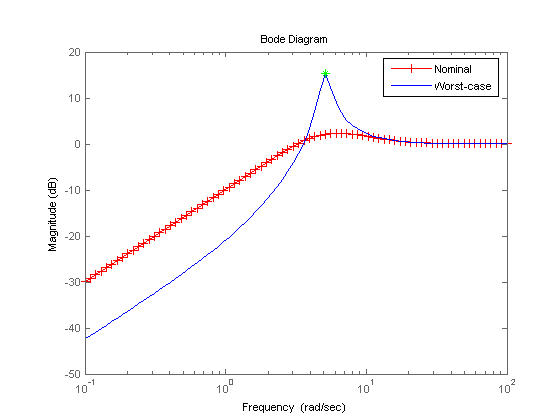
Finally, plot Bode magnitude plots of the nominal and worst-case values of the sensitivity function. Observe that the peak value of Sworst occurs at the frequency maxgain.CriticalFrequency.

bodemag(Sg.NominalValue,'r-+',Sgworst,'b');
legend('Nominal','Worst-case')
hold on
semilogx(maxgain.CriticalFrequency,20*log10(maxgain.LowerBound),'g*')
hold off