Control of F-14 Lateral Axis (mu-Synthesis)

This example shows how to use mu-analysis and synthesis tools to design a robust controller for the lateral-directional axis of the F-14 aircraft during powered approach to landing. The linearized F-14 model is found at an angle-of-attack (alpha) of 10.5 degrees and airspeed of 140 knots.

Performance Specifications
From Specs to Weighting Functions
Nominal Aircraft Model
Accounting for Modeling Errors
Building an Uncertain Model of the Aircraft Dynamics
Analyzing How Modeling Errors Affect the Open-Loop Responses
Designing the Lateral-Axis Controller
Frequency-Domain Comparison of the Controllers
Time-Domain Validation of the Robust Controller

Performance Specifications

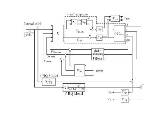
The figure below shows a block diagram of the closed-loop system. This diagram includes the nominal aircraft model, the controller K, as well as elements capturing the model uncertainty and performance objectives (see next sections for details).

f14icpic = imread('F14ICdiagram.jpg');
image(f14icpic);
set(gca,'Visible','off')

        Robust Control Design for F-14 Lateral Axis

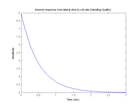
The design goal is to have the "true" airplane respond effectively to the pilot's lateral stick and rudder pedal inputs. These performance specifications include:

Decoupled responses from lateral stick to roll rate p and from rudder pedals to side-slip angle beta. The lateral stick and rudder pedals have a maximum deflection of +/- 1 inch.

The aircraft handling quality (HQ) response from lateral stick to roll rate p should match the first-order response

   hq_p    = 5.0 * tf(2.0,[1 2.0]);
   step(hq_p), title('Desired response from lateral stick to roll rate (Handling Quality)')

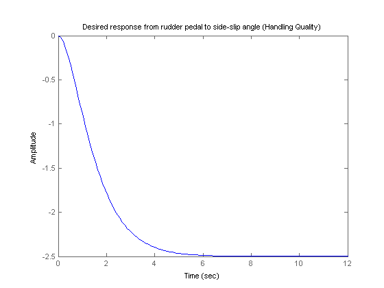
The aircraft handling quality response from the rudder pedals to the side-slip angle beta should should match the damped second-order response

   hq_beta = -2.5 * tf(1.25^2,[1 2.5 1.25^2]);
   step(hq_beta), title('Desired response from rudder pedal to side-slip angle (Handling Quality)')

The stabilizer actuators have +/- 20 degs and +/- 90 degs/sec limits on their deflection and deflection rate. The rudder actuators have +/- 30 degs and +/-125 degs/sec deflection and deflection rate limits.

The three measurement signals ( roll rate p, yaw rate r, and lateral acceleration y_ac ) are filtered through second-order anti-aliasing filters:

   freq = 12.5 * (2*pi);  % 12.5 Hz
   zeta = 0.5;
   antia_filt_yaw = tf(freq^2,[1 2*zeta*freq freq^2]);
   antia_filt_lat = tf(freq^2,[1 2*zeta*freq freq^2]);

   freq = 4.1 * (2*pi);  % 4.1 Hz
   zeta = 0.7;
   antia_filt_roll = tf(freq^2,[1 2*zeta*freq freq^2]);

   antia_filt = append(antia_filt_roll,antia_filt_yaw,antia_filt_lat);

From Specs to Weighting Functions

H_infinity design algorithms seek to minimize the largest closed-loop gain across frequency (H_infinity norm). To apply these tools, you must first recast your design tradeoffs and frequency-dependent specifications as constraints on the closed-loop gains. You can do this by using weighting functions to "normalize" your specifications across frequency and to adequately weight each requirement.

Here is how you can express the F14 specs in terms of weighting functions:

To capture the limits on the actuator deflection magnitude and rate, pick a diagonal, constant weight W_act corresponding to the stabilizer and rudder deflection rate and deflection limits.

    W_act = diag([1/90,1/20,1/125,1/30]);

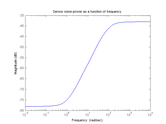
Use a 3x3 diagonal, high-pass filter W_n to model the frequency content of the sensor noise in the roll rate, yaw rate, and lateral acceleration channels.

    W_n = append(0.025,tf(0.0125*[1 1],[1 100]),0.025);
    clf, bodemag(W_n(2,2)), title('Sensor noise power as a function of frequency')

The lateral stick-to-p and rudder pedal-to-beta responses should match the handling quality targets hq_p and hq_beta. This is a model matching objective: you want to minimize the difference (peak gain) between the desired and actual closed-loop transfer functions. Performance is limited due to a right-half plane zero in the model at 0.002 rad/sec, so accurate tracking of sinusoids below 0.002 rad/sec isn't possible. Accordingly, weight the first handling quality spec with a bandpass filter W_p that emphasizes the frequency range between 0.06 and 30 rad/sec (a roll rate tracking error of less than 5% is desired).

    W_p = tf([0.05 2.9 105.93 6.17 0.16],[1 9.19 30.80 18.83 3.95]);
    clf, bodemag(W_p), title('Weight on Handling Quality spec')

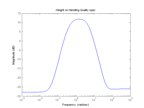
Similarly, pick W_beta=2*W_p for the second handling quality spec

    W_beta = 2*W_p;

Here the weights W_act, W_n, W_p, and W_beta have been scaled so that the closed-loop gain between all external inputs and all weighted outputs is less than 1 at all frequencies.

Nominal Aircraft Model

The pilot can command the lateral-directional response of the aircraft with the lateral stick and rudder pedals. The aircraft has:

Two control inputs: differential stabilizer deflection (delta_dstab, degrees) and rudder deflection (delta_rud, degrees).
Three measured outputs: roll rate (p, deg/sec), yaw rate (r, degs/sec), and lateral acceleration (y_ac, g's).
One calculated output: side-slip angle (beta).

The nominal lateral directional F-14 model, F14nominal, has four states: lateral velocity (v), yaw rate (r), roll rate (p), and roll angle (phi). These variables are related by the state space equations:

where x = [v; r; p; phi], u = [delta_dstab; delta_rud], and y = [beta; p; r; y_ac].

load F14nominal
F14nominal

 
a = 
                 Lateral Velo   Yaw Rate (r  Roll Rate (p  Roll Angle (
   Lateral Velo        -0.116        -227.3         43.02         31.63
   Yaw Rate (r        0.00265        -0.259       -0.1445             0
   Roll Rate (p      -0.02114        0.6703        -1.365             0
   Roll Angle (             0        0.1853             1             0
 
 
b = 
                 Differential  Rudder (deg)
   Lateral Velo        0.0622        0.1013
   Yaw Rate (r      -0.005252      -0.01121
   Roll Rate (p      -0.04666      0.003644
   Roll Angle (             0             0
 
 
c = 
                 Lateral Velo   Yaw Rate (r  Roll Rate (p  Roll Angle (
   Sideslip (be        0.2469             0             0             0
   Roll Rate (p             0             0          57.3             0
   Yaw Rate (r              0          57.3             0             0
   lateral acce     -0.002827     -0.007877       0.05106             0
 
 
d = 
                 Differential  Rudder (deg)
   Sideslip (be             0             0
   Roll Rate (p             0             0
   Yaw Rate (r              0             0
   lateral acce      0.002886      0.002273
 
Continuous-time model.

The complete airframe model also includes actuators models A_S and A_R. The actuator outputs are their respective rates and deflections. The actuator rates are used to penalize actuation effort.

A_S = [tf([25 0],[1 25]); tf(25,[1 25])];
A_R = A_S;

Accounting for Modeling Errors

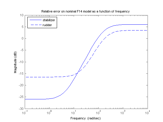
The nominal F14 model only approximates the "true" airplane behavior. To account for unmodeled dynamics, you can introduce a relative error term or multiplicative uncertainty | W_in * Delta_G | at the plant input, where the error dynamics Delta_G have gain less than 1 across frequencies, and the weighting function W_in reflects in what frequency ranges the model is more or less accurate. Because there is typically more modeling errors at high frequency so W_in is high pass.

% Normalized error dynamics
Delta_G = ultidyn('Delta_G',[2 2],'Bound',1.0);

% Frequency shaping of error dynamics
w_1 = tf(2.0*[1 4],[1 160]);
w_2 = tf(1.5*[1 20],[1 200]);
W_in = append(w_1,w_2);

bodemag(w_1,'-',w_2,'--')
title('Relative error on nominal F14 model as a function of frequency')
legend('stabilizer','rudder','Location','NorthWest');

Building an Uncertain Model of the Aircraft Dynamics

Now that you quantified modeling errors, you can build an uncertain model of the aircraft dynamics corresponding to the dashed box in the figure below

f14icpic = imread('F14ICdiagram.jpg');
image(f14icpic);
set(gca,'Visible','off')

Use the sysic command to combine the nominal airframe model F14nominal, the actuator models A_S and A_R, and the modeling error description W_in * Delta_G into a single uncertain model mapping [delta_dstab; delta_rud] to the plant and actuator outputs:

systemnames = 'F14nominal A_S A_R W_in Delta_G';
inputvar = '[delta_dstab; delta_rud]';
outputvar = '[A_S; A_R; F14nominal]';
input_to_F14nominal = '[A_S(2); A_R(2)]';
input_to_A_S = '[delta_dstab + W_in(1)]';
input_to_A_R = '[delta_rud + W_in(2)]';
input_to_W_in = '[Delta_G]';
input_to_Delta_G = '[delta_dstab; delta_rud]';
sysoutname = 'F14_unc';
cleanupsysic = 'yes';
echo off; sysic; echo on

This produces an uncertain state-space (USS) model F14_unc of the aircraft:

F14_unc

USS: 8 States, 8 Outputs, 2 Inputs, Continuous System
  Delta_G: 2x2 LTI, max. gain = 1, 1 occurrence

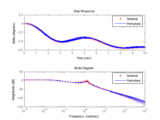
Analyzing How Modeling Errors Affect the Open-Loop Responses

You can analyze the effect of modeling uncertainty by picking random samples of the unmodeled dynamics Delta_G and plotting the nominal and perturbed time responses (Monte Carlo analysis). For example, for the differential stabilizer channel, the uncertainty weight w_1 implies a 5% modeling error at low frequency, increasing to 100% after 93 rad/sec, as confirmed by the Bode diagram below.

% Pick 10 random samples
F14_unc_sampl = usample(F14_unc,10);

% Look at response from differential stabilizer to beta
clf
subplot(211), step(F14_unc.Nominal(5,1),'r+',F14_unc_sampl(5,1),'b-',10)
legend('Nominal','Perturbed'),ylabel('Beta (degrees)')

subplot(212), bodemag(F14_unc.Nominal(5,1),'r+',F14_unc_sampl(5,1),'b-',{0.001,1e3})
legend('Nominal','Perturbed')

Designing the Lateral-Axis Controller

You can now proceed with designing a controller that robustly achieves the specifications (here "robustly" means for any perturbed aircraft model consistent with the modeling error bounds W_in).

First build an open-loop model F14IC mapping the external input signals to the performance-related outputs (see figure below).

clf
f14genicpic = imread('F14_generalplant.jpg');
image(f14genicpic);
set(gca,'position',[.1 .25 .8 .5],'Visible','off')

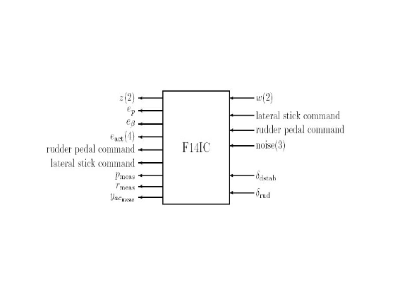
Again you can use sysic to build F14IC:

systemnames = 'F14_unc antia_filt hq_p hq_beta ';
systemnames = [systemnames ' W_act W_n W_p W_beta'];
inputvar  = '[sn_nois{3}; roll_cmd; beta_cmd; delta_dstab; delta_rud]';
outputvar = '[ W_p; W_beta; W_act;  roll_cmd; beta_cmd; antia_filt + W_n ]';
input_to_F14_unc       = '[ delta_dstab; delta_rud ]';
input_to_antia_filt = '[ F14_unc(6:8) ]';
input_to_hq_beta = '[ beta_cmd ]';
input_to_hq_p    = '[ roll_cmd ]';
input_to_W_act      = '[ F14_unc(1:4) ]';
input_to_W_beta     = '[ hq_beta - F14_unc(5) ]';
input_to_W_p        = '[ hq_p - F14_unc(6) ]';
input_to_W_n        = '[ sn_nois ]';
sysoutname = 'F14IC';
cleanupsysic = 'yes';
sysic

This produces the uncertain state-space model

F14IC

USS: 26 States, 11 Outputs, 7 Inputs, Continuous System
  Delta_G: 2x2 LTI, max. gain = 1, 1 occurrence

Recall that by construction of the weighting functions, a controller meets the specs whenever the closed-loop gain is less than 1 at all frequencies and for any I/O directions. You can first design an H-infinity controller that minimizes the closed-loop gain for the nominal aircraft model:

nmeas = 5;		% number of measurements
nctrls = 2;		% number of controls
[kinf,ginf,gammainf] = hinfsyn(F14IC.NominalValue,nmeas,nctrls);
gammainf

gammainf =
    0.6708

Here hinfsyn computed a controller kinf that keeps the closed-loop gain below gammainf = 0.67 < 1, so the specs can be met for the nominal aircraft model.

Next perform a mu-synthesis to see if the specs can be met robustly when taking into account the modeling errors (uncertainty Delta_G). We use the command dksyn to perform the synthesis and set the frequency grid used for mu-analysis and the number of D-K iterations with dkitopts.

fmu = logspace(-2,2,60);
opt = dkitopt('FrequencyVector',fmu,'NumberofAutoIterations',5);
[kmu,clpmu,bnd] = dksyn(F14IC,nmeas,nctrls,opt);
bnd

bnd =
    1.2322

Here the best controller kmu could only keep the closed-loop gain below bnd = 1.23 for the specified model uncertainty, indicating that the specs can be nearly but not fully met for the family of aircraft models under consideration.

Frequency-Domain Comparison of the Controllers

Let's compare the performance and robustness of the H-infinity controller kinf and mu controller kmu. Recall that the performance specs are achieved when the closed loop gain is less than 1 for every frequency.

First use the lft command to close the loop around each controller:

clinf = lft(F14IC,kinf);
clmu = lft(F14IC,kmu);

To facilitate the analysis, sample the frequency response of the uncertain closed-loop model over the frequency grid fmu, thus creating an uncertain frequency response or UFRD:

clinfg = frd(clinf,fmu)
clmug = frd(clmu,fmu)

UFRD: 6 Outputs, 5 Inputs, Continuous System, 60 Frequency points
  Delta_G: 2x2 LTI, max. gain = 1, 1 occurrence
UFRD: 6 Outputs, 5 Inputs, Continuous System, 60 Frequency points
  Delta_G: 2x2 LTI, max. gain = 1, 1 occurrence

What is the worst-case performance (in terms of closed-loop gain) of each controller for modeling errors bounded by W_in? The wcgain command helps you answer this difficult question directly without need for extensive gridding and simulation.

opt=wcgopt('FreqPtWise',1);  % options for WCGAIN

% Compute worst-case gain (as a function of frequency) for kinf
[mginf,wcuinf] = wcgain(clinfg,opt);
mginf

mginf = 
           LowerBound: [1x1 frd]
           UpperBound: [1x1 frd]
    CriticalFrequency: 1.2638

% Compute worst-case gain for kinf
[mgmu,wcumu,infomu] = wcgain(clmug,opt);
mgmu

mgmu = 
           LowerBound: [1x1 frd]
           UpperBound: [1x1 frd]
    CriticalFrequency: 0.4238

You can now compare the nominal and worst-case performance (peak gain<1) for each controller:

clf
subplot(211)
semilogx(fnorm(clinfg.NominalValue),'r',mginf.UpperBound,'b');
title('Performance analysis for kinf')
xlabel('Frequency (rad/sec)')
ylabel('Closed-loop gain');
legend('Nominal Plant','Worst-Case','Location','NorthWest');

subplot(212)
semilogx(fnorm(clmug.NominalValue),'r',mgmu.UpperBound,'b');
title('Performance analysis for kmu')
xlabel('Frequency (rad/sec)')
ylabel('Closed-loop gain');
legend('Nominal Plant','Worst-Case','Location','SouthWest');

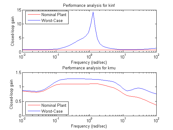
The first plot shows that while the H-infinity controller kinf meets the performance specs for the nominal plant model, its performance can sharply deteriorate (peak gain near 15) for some perturbed model within our modeling error bounds.

In contrast, the mu controller kmu has slightly worse performance for the nominal plant when compared to kinf, but it maintains this performance consistently for all perturbed models (worst-case gain near 1.25). The mu controller is therefore more robust to modeling errors.

Time-Domain Validation of the Robust Controller

To further test the robustness of the mu controller kmu in the time domain, you can compare the time responses of the nominal and worst-case closed-loop models with the ideal "Handling Quality" response. To do this, first construct the "true" closed-loop model F14SIM where all weighting functions and HQ reference models have been removed:

systemnames = 'F14_unc antia_filt kmu';
inputvar  = '[roll_cmd; beta_cmd]';
outputvar = '[F14_unc(6); F14_unc(5)]';
input_to_F14_unc       = '[ kmu ]';
input_to_antia_filt = '[ F14_unc(6:8) ]';
input_to_kmu = '[ roll_cmd; beta_cmd; antia_filt ]';
sysoutname = 'F14SIM';
cleanupsysic = 'yes';
sysic
F14SIM.OutputName = {'Roll rate (deg/sec)','Side-slip angle (deg)'};

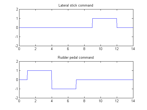
Next, create the test signals u_stick and u_pedal shown below

time = 0:0.02:15;
u_stick = (time>=9 & time<12);
u_pedal = (time>=1 & time<4) - (time>=4 & time<7);

clf
subplot(211), plot(time,u_stick), axis([0 14 -2 2]), title('Lateral stick command')
subplot(212), plot(time,u_pedal), axis([0 14 -2 2]), title('Rudder pedal command')

You can now compute and plot the ideal, nominal, and worst-case responses to the test commands u_stick and u_pedal

% Ideal behavior
F14ideal = append(hq_p,hq_beta);

% Find frequency where worst-case gain occurs
% and apply corresponding worst-case perturbation
wcfreqidx = find(mgmu.CriticalFrequency==infomu.Frequency);
F14wc = usubs(F14SIM,wcumu{wcfreqidx});

% Compare responses
clf
lsim(F14ideal,'g',F14SIM.NominalValue,'r',F14wc,'b--',[u_stick ; u_pedal],time)
legend('ideal','nominal','perturbed','Location','SouthEast');
title('Closed-loop responses with mu controller KMU')

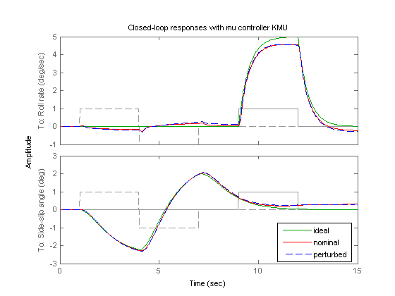
The closed-loop response is nearly identical for the nominal and worst-case closed-loop systems. Note that the roll-rate response of the F-14 tracks the roll-rate command well initially and then departs from this command. This is due to a right-half plane zero in the aircraft model at 0.024 rad/sec.