
This demonstrates how to design a multi-input, multi-output controller by shaping the gain of the open-loop response across frequency. This technique is applied to controlling the pitch axis of a HIMAT aircraft.
You will see how to choose a suitable target loop shape and then use the loopsyn command to compute a multivariable controller that optimally matches the target loop shape.
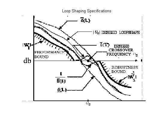
Typically, loop shaping is a tradeoff between two potentially conflicting objectives. You want to maximize the open-loop gain to get the best possible performance, but for robustness you need to drop the gain below 0dB where the model accuracy is poor and high gain might cause instabilities. This requires a good model where performance is needed (typically at low frequencies), and sufficient roll-off at higher frequencies where the model is often poor. The frequency Wc where the gain crosses the 0dB line is called the crossover frequency and marks the transition between performance and robustness requirements.
This tradeoff between performance and robustness leads to the typical loop shape shown below:
[fig1,mapp]=imread('loopsyn_demo1','png');image(fig1);
colormap(mapp);axis off image;
title('Loop Shaping Specifications')
Guidelines for choosing your target loop shape Gd includes
A simple target loop shape is
where the crossover Wc is simply the reciprocal of the rise-time of the desired step response.
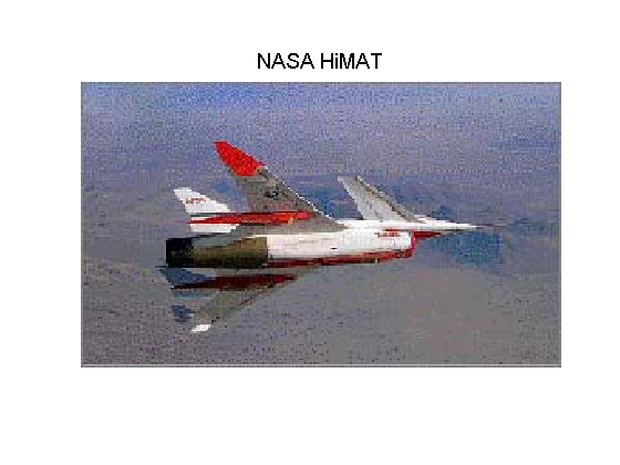
For illustration purposes we use a six-state model of the longitudinal dynamics of the HiMAT aircraft trimmed at 25000 ft and 0.9 Mach. The aircraft dynamics are unstable, with two right half plane phugoid modes.
[fig0,mapp]=imread('loopsyn_demo0','jpg');image(fig0);
colormap(mapp);axis off image;
title('NASA HiMAT','FontSize',14)
This model has two control inputs:
and two measured outputs:
The model is unreliable beyond 100 rad/sec. Fuselage bending modes and other uncertain factors induces deviations between to model and the true aircraft of as much as 20 decibels (or 1000%) beyond frequency 100 rad/sec.
ag =[
-2.2567e-02  -3.6617e+01  -1.8897e+01  -3.2090e+01   3.2509e+00  -7.6257e-01;
9.2572e-05  -1.8997e+00   9.8312e-01  -7.2562e-04  -1.7080e-01  -4.9652e-03;
1.2338e-02   1.1720e+01  -2.6316e+00   8.7582e-04  -3.1604e+01   2.2396e+01;
0            0   1.0000e+00            0            0            0;
0            0            0            0  -3.0000e+01            0;
0            0            0            0            0  -3.0000e+01];
bg = [0     0;
      0     0;
      0     0;
      0     0;
     30     0;
      0    30];
cg = [0     1     0     0     0     0;
      0     0     0     1     0     0];
dg = [0     0;
      0     0];
G=ss(ag,bg,cg,dg);
G.InputName = {'elevon','canard'};
G.OutputName = {'alpha','theta'};

clf
step(G), title('Open-loop step response of HIMAT aircraft')

Your task is to control alpha and theta by issuing appropriate elevon and canard commands. You also want minimum spillover between channels, that is, a command in alpha should have minimum effect on theta and vice versa.
Designing a controller with loopsyn involves the following steps:
The aircraft model G has two unstable right-half plane phugoid mode poles. It has one zero, which is in the left-half plane:
plant_poles=pole(G), plant_zeros=zero(G)
plant_poles =
  -5.6757
   0.6898 + 0.2488i
   0.6898 - 0.2488i
  -0.2578
 -30.0000
 -30.0000
plant_zeros =
   -0.0210
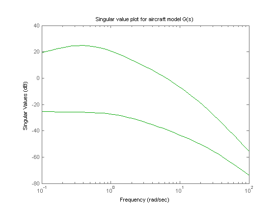
Use sigma to plot the min and max I/O gain as a function of frequency:
clf, sigma(G,'g',{.1,100});
title('Singular value plot for aircraft model G(s)');
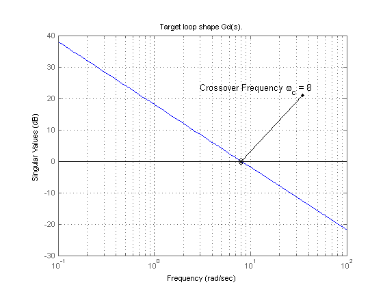
For this design we use the target loop shape Gd(s)=8/s corresponding to a rise time of about 1/8=0.125 sec.
s=zpk('s'); % Laplace variable s
Gd=8/s;
sigma(Gd,{.1 100}), grid, title('Target loop shape Gd(s).')

% create textarrow pointing to crossover frequency Wc
hold on;
plot([8,35],[0,21],'k.-');plot(8,0,'kd');
plot([.1,100],[0 0],'k');
text(3,23,'Crossover Frequency \omega_c = 8');
hold off;
You are now ready to design an H-infinity controller K such that the gains of the open-loop response G(s)*K(s) matches the target loop shape Gd as well as possible (while stabilizing the aircraft dynamics).
[K,CL,GAM] = loopsyn(G,Gd);
GAM
GAM =
    1.6445
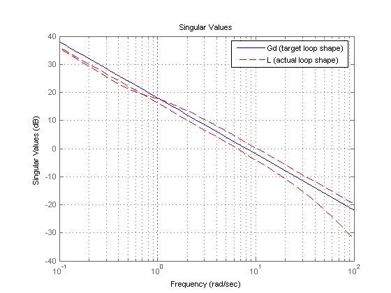
The value GAM=1.64 indicates that the target loop shape was meet within +/-4.3dB (using 20*log10(GAM)=4.32). Compare the singular values of the open-loop L=G*K with the target loop shape Gd
L=G*K;              % form the compensated loop L
sigma(Gd,'b',L,'r--',{.1,100});grid
legend('Gd (target loop shape)','L (actual loop shape)');
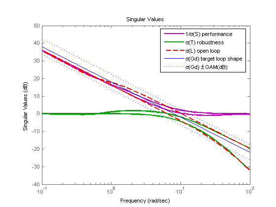
Next compare the gains of the open-loop transfer L, closed-loop transfer T, and sensitivity function S.
T = feedback(L,eye(2));
T.InputName = {'alpha command','theta command'};
S = eye(2)-T;

% SIGMA frequency response plots
sigma(inv(S),'m',T,'g',L,'r--',Gd,'b',Gd/GAM,'b:',...
	Gd*GAM,'b:',{.1,100})
legend('1/\sigma(S) performance',...
	'\sigma(T) robustness',...
	'\sigma(L) open loop',...
	'\sigma(Gd) target loop shape',...
	'\sigma(Gd) \pm GAM(dB)');
% make lines fatter and fonts larger
set(findobj(gca,'Type','line','-not','Color','b'),'LineWidth',2);
Finally, plot the step responses of the closed-loop system T
step(T,8)
title('Responses to step commands for alpha and theta');
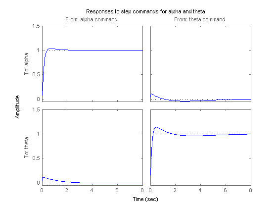
Your design looks good. The alpha and theta controls are fairly decoupled, overshoot is less the 15 percent, and peak time is only 0.5 sec.
You just designed a 2-input, 2-output controller K with satisfactory performance. However this controller has fairly high order:
size(K)
State-space model with 2 outputs, 2 inputs, and 16 states.
You can now use model reduction algorithms to try to simplify this controller while retaining its performance characteristics. First compute the Hankel singular values of K to understand how many controller states effectively contribute to the control law:
[Kb,hsv] = balreal(K);
semilogy(hsv,'r-*'), grid
title('Hankel singular values of K'), xlabel('Order')
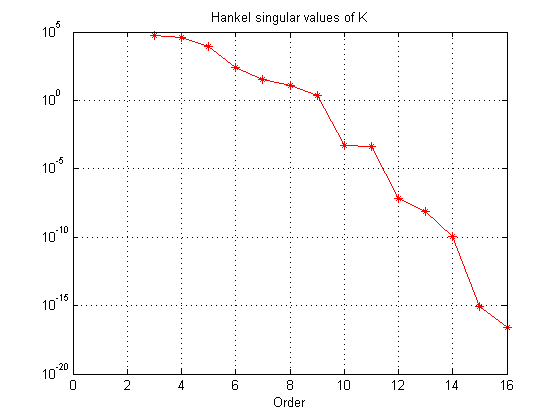
The Hankel singular values hsv measure the relative energy of each state in the balanced realization Kb. Notice that hsv drops by 3 orders of magnitude between the 9th and 10th state, so try discarding the states 10 through 16.
Kr = modred(Kb,10:16);
size(Kr)
State-space model with 2 outputs, 2 inputs, and 9 states.
The simplified controller Kr has order 9 compared to 16 for the initial controller K. Compare the approximation error K-Kr across frequency with the gains of K.
sigma(K,'b',K-Kr,'r-.')
legend('K','error K-Kr')
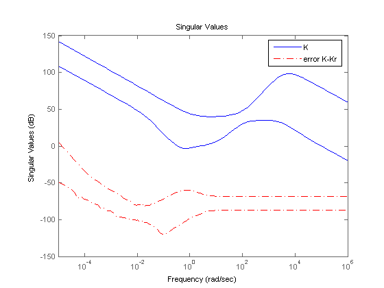
This plot suggests that the approximation error is small in relative terms, so go ahead and compare the closed-loop responses with the original and simplified controllers K and Kr
Tr = feedback(G*Kr,eye(2));
step(T,'b',Tr,'r-.',8)
title('Responses to step commands for alpha and theta');
legend('K','Kr')
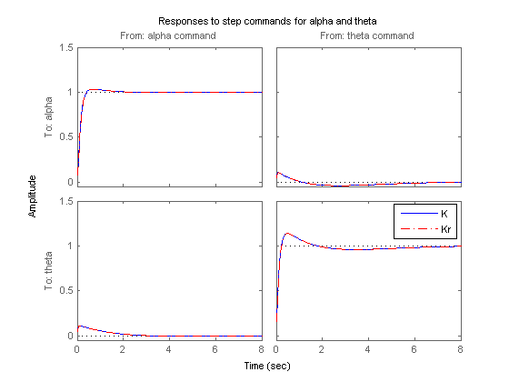
The two responses are indistinguishable so your simplified 9th-order controller Kr is a good substitute for K for implementation purposes.