Simplifying Higher-Order Plant Models

This demo shows how you can approximate high-order plant models by simpler, low-order models using the tools available in the Robust Control Toolbox.

Motivation
The Model Reduction Process
Example: A Model for Rigid Body Motion of a Building
Examining the Plant Dynamics
Computing Hankel Singular Values
Performing Model Reduction using an Additive Error Bound
Performing Model Reduction using a Multiplicative Error Bound
Validating the Results
Picking the Lowest Order Compatible with a Desired Accuracy Level
References

Motivation

There are situations where you have to deal with models that are quite large:

High-Order Plants: Detailed first-principles or finite-element models of your plant tend to have high order. It is often desirable to simplify such models for simulation or control design purposes.

High-Order Controllers: Robust control techniques often yield high-order controllers. This is common, e.g., when frequency weighting functions are used for shaping the open-loop response. It is often desirable to simplify such controllers for implementation purposes.

For control purposes, it is generally enough to have an accurate model near the crossover frequency. For simulation purposes, it is enough to capture the essential dynamics in the frequency range of the excitation signals. This means that it is often possible to find low-order approximations of high-order models. The Robust Control Toolbox offers a variety of model reduction algorithms to best suit your requirements and your model characteristics.

The Model Reduction Process

A model reduction task typically involves the following steps:

Analyze the important characteristics of the model from its time- or frequency-domain responses using, e.g., step or bode
Determine an appropriate reduced order by plotting the Hankel singular values of the original model (hankelsv) to determine which modes (states) can be discarded without sacrificing the key characteristics.
Choose a reduction algorithm. The various reduction methods available in the toolbox are: balancmr, bstmr, schurmr, hankelmr, and ncfmr. You can easily access these algorithms through the top-level interface reduce. The methods employ different measures of "closeness" between the original and reduced models. The choice is application dependent. You may try all of them to investigate their relative merits.
Validation: Validate your results by comparing the dynamics of the reduced model to the original. You may need to adjust your reduction parameters (choice of model order, algorithm, error bounds etc.) if the results are not satisfactory.

Example: A Model for Rigid Body Motion of a Building

Let us see how to apply the reduction methods on a model of a building. The building (the Los Angeles University Hospital) has 8 floors, each considered as having 3 degrees of freedom - two displacements and one rotation. We can represent the input-output relationship for any one of these displacements using a 48-state model, where each state represents a displacement or its rate of change (velocity).

load build.mat

Examining the Plant Dynamics

Let us begin by analyzing the frequency response of the model.

bode(G)
grid on

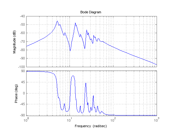
As observed from the frequency response of the model, the essential dynamics of the system lie in the frequency range of 3 to 50 rad/s. The magnitude drops in both the very low as well has the high frequency ranges. Your objective is to find a low-order model that preserves the information content in this frequency range to an acceptable level of accuracy.

Computing Hankel Singular Values

In order to gain insight into what states of the model can be safely discarded, look at the Hankel singular values of the model.

hsv_add = hankelsv(G);
bar(hsv_add)
title('Hankel Singular Values of the Model (G)');
xlabel('Number of States')
ylabel('Singular Values (\sigma_i)')
line([10.5 10.5],[0 1.5e-3],'Color','r','linestyle','--','linewidth',1)
text(6,1.6e-3,'10 dominant states.')

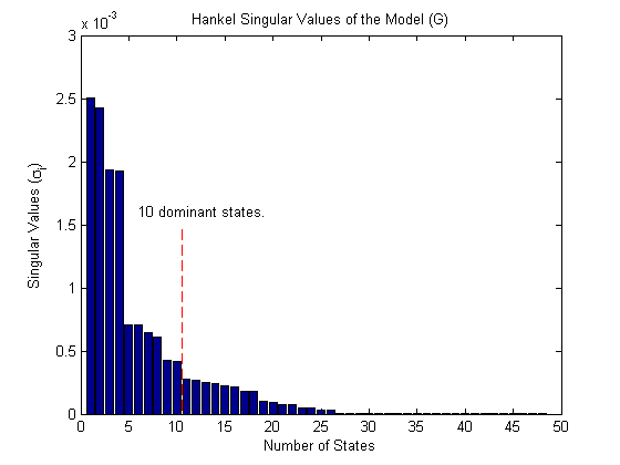
The Hankel singular value plot suggests that there are 4 dominant modes in this system. However, the contribution of the remaining modes is still significant. Let us draw the line at 10 states and discard the remaining ones. In other words, let's try to find a 10th-order reduced model Gr that best approximates the original system G.

Performing Model Reduction using an Additive Error Bound

The function reduce is the gateway to all model reduction routines available in the toolbox. Let us use the default, Square-root Balance Truncation ('balancmr') option of reduce as the first step. This method uses an "additive" error bound for reduction, meaning that it tries to keep the absolute approximation error uniformly small across frequencies.

% Compute 10th-order reduced model (reduce uses balancmr method by default)
[Gr_add,info_add] = reduce(G,10);

% Now compare the original model G to the reduced model Gr_add
bode(G,'b',Gr_add,'r'), grid on
title('Comparing Original (G) to the Reduced model (Gr\_add)')
legend('G - 48-state original ','Gr\_add - 10-state reduced','location','northeast')

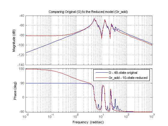
Performing Model Reduction using a Multiplicative Error Bound

As seen from the Bode plot above, the reduced model captures the resonances below 30 rad/s quite well, but the match in the low frequency region (<2 rad/s) is poor. Also, the reduced model does not fully capture the dynamics in the 30-50 rad/s frequency range. A possible explanation for large errors at low frequencies is the relatively low gain of the model at these frequencies. Consequently, even large errors at these frequencies contribute little to the overall error.

To get around this problem, try a multiplicative-error method like bstmr. This algorithm emphasizes relative errors rather than absolute ones. Because relative comparisons do not work when gains are close to zero, you need to add a minimum-gain threshold, e.g., by adding a feedthrough gain d to your original model. Assuming you are not concerned about errors at gains below -100 dB, you can set the feedthrough to 1e-5.

GG = G;
GG.d = 1e-5;

Now look at the singular values for multiplicative (relative) errors (use 'mult' option of hankelsv)

hsv_mult = hankelsv(GG,'mult');
bar(hsv_mult)
title('Multiplicative-Error Singular Values of the Model (G)');
xlabel('Number of States')
ylabel('Singular Values (\sigma_i)')

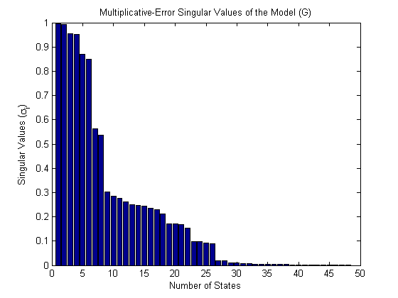
A 26th-order model looks promising, but for sake of comparison with the previous result, we stick to a 10th order reduction.

% Use bstmr algorithm option for model reduction
[Gr_mult,info_mult] = reduce(GG,10,'algorithm','bst');

%now compare the original model G to the reduced model Gr_mult
bode(G,Gr_add,Gr_mult,{1e-2,1e4}), grid on
title('Comparing Original (G) to the Reduced models (Gr\_add and Gr\_mult)')
legend('G - 48-state original ','Gr\_add (balancmr)','Gr\_mult (bstmr)','location','northeast')

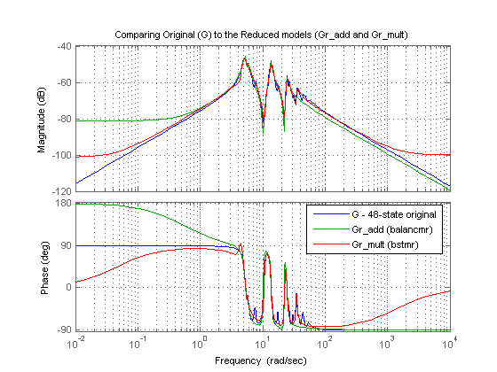
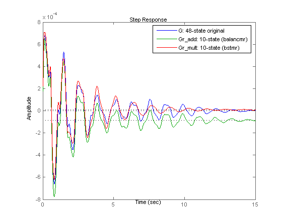
The fit between the original and the reduced model is much better with the multiplicative-error approach, even at low frequencies. This is confirmed by comparing the step responses:

step(G,Gr_add,Gr_mult,15) %step response until 15 seconds
legend('G: 48-state original ','Gr\_add: 10-state (balancmr)','Gr\_mult: 10-state (bstmr)')

Validating the Results

All algorithms provide bounds on the approximation error. For additive-error methods like balancmr, the approximation error is measured by the peak (maximum) gain of the error model G-Greduced across all frequencies. This peak gain is also known as the H-infinity norm of the error model. The error bound for additive-error algorithms looks like

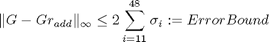
where the sum is over all discarded Hankel singular values of G (entries 11 through 48 of hsv_add). You can verify that this bound is satisfied by comparing the two sides of this inequality:

norm(G-Gr_add,inf) % actual error

% theoretical bound (stored in the "ErrorBound" field of the "INFO"
% struct returned by |reduce|)
info_add.ErrorBound

ans =
  6.0154e-004
ans =
    0.0047

For multiplicative-error methods like bstmr, the approximation error is measured by the peak gain across frequency of the relative error model G\(G-Greduced), and the error bound looks like

where the sum is over the discarded multiplicative Hankel singular values computed by hankelsv(G,'mult'). Again compare these bounds for the reduced model Gr_mult

norm(GG\(GG-Gr_mult),inf) % actual error

% Theoretical bound
info_mult.ErrorBound

ans =
    0.5949
ans =
  473.2954

Plot the relative error for confirmation

bodemag(GG\(GG-Gr_mult),{1e-2,1e3})
grid on
text(0.1,-50,'Peak Gain: -4.6 dB (59%) at 17.2 rad/s')
title('Relative error between original model (G) and reduced model (Gr\_mult)')

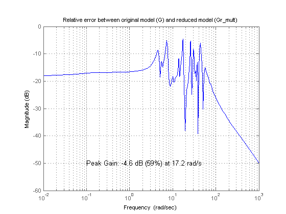
From the relative error plot above, there is up to 59% relative error at 17.2 rad/s, which may be more than you are willing to accept.

Picking the Lowest Order Compatible with a Desired Accuracy Level

To improve the accuracy of Gr_mult, you need to increase the order. If you want at least 5% relative accuracy, what is the lowest order you can get? The function reduce can automatically select the lowest-order model compatible with your desired level of accuracy.

% Specify a maximum of 5% approximation error
[Gred,info] = reduce(GG,'ErrorType','mult','MaxError',0.05);
size(Gred)

State-space model with 1 output, 1 input, and 34 states.

The algorithm has picked a 34-state reduced model Gred. Compare the actual error with the theoretical bound:

norm(GG\(GG-Gred),inf)
info.ErrorBound

ans =
    0.0068
ans =
    0.0423

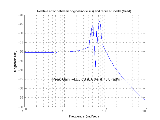
Look at the relative error magnitude as a function of frequency. Higher accuracy has been achieved at the expense of a larger model order (from 10 to 34). Note that the actual maximum error is 0.6%, much less than the 5% target. This discrepancy comes from the fact that bstmr uses the error bound rather than the actual error to select the order.

bodemag(GG\(GG-Gred),{1,1e3})
grid on
text(5,-75,'Peak Gain: -43.3 dB (0.6%) at 73.8 rad/s')
title('Relative error between original model (G) and reduced model (Gred)')

Compare the Bode responses

bode(G,Gred,{1e-2,1e4}), grid on
legend('G - 48-state original','Gred - 34-state reduced')

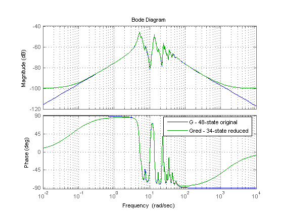
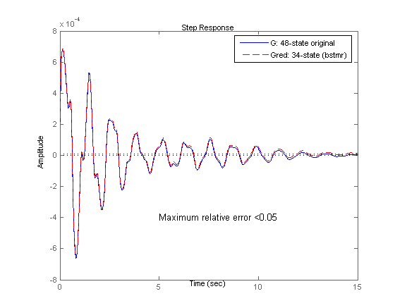
Finally, compare the step responses of the original and reduced models. They are virtually indistinguishable.

step(G,'b',Gred,'r--',15) %step response until 15 seconds
legend('G: 48-state original ','Gred: 34-state (bstmr)')
text(5,-4e-4,'Maximum relative error <0.05')

References

The example discussed here was taken from the "Benchmark examples for model reduction of linear time invariant dynamical systems" available at: http://www.win.tue.nl/niconet/NIC2/benchmodred.html.