This demo shows how to analyze and quantify the robustness of feedback control systems to modeling errors and parameter variations. You will learn how to test for robust stability with robuststab and gain insight into the connection with mu analysis and the mussv command.
Figure 1 shows the block diagram of the closed-loop system under consideration. The plant model P is uncertain, the signals d and n are disturbances, and e must be kept small for adequate disturbance rejection.
image(imread('mudemo1.tif')); axis off image
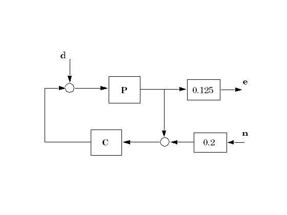
Figure 1. Closed-Loop System for Robustness Analysis
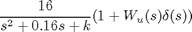
The uncertain plant model is a lightly-damped, second-order system with parametric uncertainty in the denominator coefficients and significant frequency-dependent umodeled dynamics beyond 6 radians/second. The mathematical model is
The parameter k is assumed to be about 40% uncertain, with a nominal value of 16. The frequency-dependent uncertainty at the plant input is assumed to be about 20% at low frequency, rising to 100% at 6 radians/second. Create and combine uncertain elements to construct the uncertain plant model, P.
k = ureal('k',16,'Percentage',40);
delta = ultidyn('delta',[1 1]);
Wu = makeweight(0.2,6,10);
P = tf(16,[1 0.16 k])*(1+Wu*delta);
For this example we use the following third-order controller:
num = [ -12.56 17.32 67.28];
den = [ 1 20.37 136.74 179.46];
C = tf(num,den);
To build an uncertain model of the closed-loop system, write the interconnection equations directly from the block diagram in Figure 1 and use sysic to compute the interconnection:
systemnames = 'P C';
inputvar = '[d; n]';
input_to_P = '[d + C]';
input_to_C = '[P + 0.2*n]';
outputvar = '[0.125*P]';
cleanupsysic = 'yes';
ClosedLoop = sysic;
Alternatively, you can use icsignal and iconnect to build the closed-loop model:
IC = iconnect;
d = icsignal(1);
n = icsignal(1);
y = icsignal(1);
IC.Input = [d;n];
IC.Output = [0.125*y];
IC.Equation{1} = equate(y,P*(d+C*(0.2*n+y)));
ClosedLoop = IC.System;
ClosedLoop.InputName = {'d' 'n'};
ClosedLoop.OutputName = {'e'};
The variable ClosedLoop is an uncertain system with 2 inputs and 1 output. It depends on two uncertain elements: a real parameter k and an uncertain linear, time-invariant dynamic element delta.
ClosedLoop
USS: 6 States, 1 Output, 2 Inputs, Continuous System
  delta: 1x1 LTI, max. gain = 1, 1 occurrence
      k: real, nominal = 16, variability = [-40  40]%, 1 occurrence
The nominal value of ClosedLoop is stable. The peak input/output gain of the nominal model is about 0.22.
pole(ClosedLoop.NominalValue)
norm(ClosedLoop.NominalValue,inf)
ans =
 -11.0706
  -1.8083 + 4.4576i
  -1.8083 - 4.4576i
  -4.1576
  -1.6852
 -60.9303
ans =
    0.2168
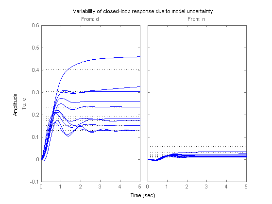
Pick 10 random samples of the uncertain closed-loop systems
clf
step(usample(ClosedLoop,10),5)
title('Variability of closed-loop response due to model uncertainty')
Does the closed-loop system remain stable for all values of k, delta in the ranges specified above? Use robuststab to answer this basic robustness question:
[stabmarg,destabunc,report,info] = robuststab(ClosedLoop);

stabmarg
stabmarg =
                UpperBound: 1.1437
                LowerBound: 1.1435
    DestabilizingFrequency: 5.8179
stabmarg gives upper and lower bounds on the robust stability margin, a measure of how much uncertainty on k, delta the feedback loop can tolerate before going unstable. For example, a margin of 0.8 indicates that as little as 80% of the specified uncertainty level can lead to instability. Here the margin is 1.14, meaning that the closed loop will remain stable for up to 114% of the specified uncertainty. report summarizes these results:
report
report =
Uncertain System is robustly stable to modeled uncertainty.
 -- It can tolerate up to 114% of modeled uncertainty.
 -- A destabilizing combination of 114% the modeled uncertainty exists,
    causing an instability at 5.82 rad/s.
 -- Sensitivity with respect to uncertain element ...
   'delta' is 100%.  Increasing 'delta' by 25% leads to a 25% decrease in the margin.
   'k' is 84%.  Increasing 'k' by 25% leads to a 21% decrease in the margin.
destabunc contains the smallest combination of (k,delta) perturbations that causes instability.
destabunc
destabunc =
    delta: [1x1 ss]
        k: 23.3197
You can substitute these values into ClosedLoop, and verify that these values causes the closed-loop system to be unstable.
pole(usubs(ClosedLoop,destabunc))
ans =
 -59.7975
 -48.5397
 -10.4942 + 8.6663i
 -10.4942 - 8.6663i
  -0.0000 + 5.8179i
  -0.0000 - 5.8179i
  -2.4292 + 1.9138i
  -2.4292 - 1.9138i
  -1.7017
Note that the natural frequency of the unstable closed-loop pole is given by stabmarg.DestabilizingFrequency.
stabmarg.DestabilizingFrequency
ans =
    5.8179
The structured singular value, or mu, is the mathematical tool used by robuststab to compute the robust stability margin. If you are comfortable with structured singular value analysis, you can use the mussv command directly to compute mu as a function of frequency and reproduce the results above. mussv is the underlying engine for all robustness analysis commands.
To use mussv, first extract the (M,Delta) decomposition of the uncertain closed-loop model ClosedLoop, where Delta is a block-diagonal matrix of (normalized) uncertain elements. The 3rd output argument of lftdata, BlkStruct, describes the block-diagonal structure of Delta and can be used directly by mussv
[M,Delta,BlkStruct] = lftdata(ClosedLoop);
For a robust stability analysis, only the channels of M associated with the uncertainty channels are used. Based on the row/column size of Delta, select the proper columns and rows of M. Remember that the rows of Delta correspond to the columns of M, and visa-versa. Consequently, the column dimension of Delta is used to specify the rows of M.
szDelta = size(Delta);
M11 = M(1:szDelta(2),1:szDelta(1));
Mu-analysis is performed on a finite grid of frequencies. For comparison purposes, evaluate the frequency response of M11 over the same frequency grid as used for the robuststab analysis.
omega = info.Frequency;
M11_g = frd(M11,omega);
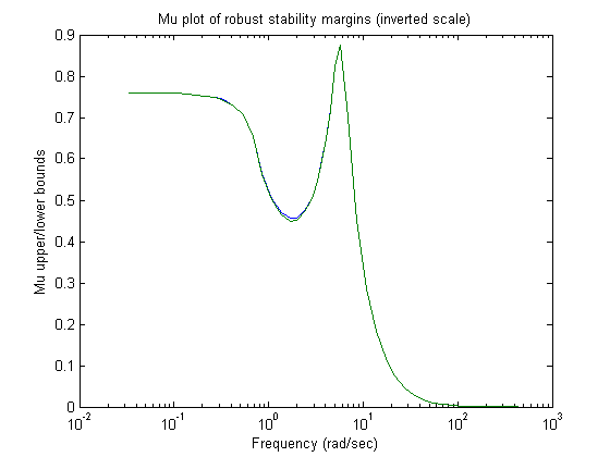
Compute mu(M11) at these frequencies and plot the resulting lower and upper bounds
mubnds = mussv(M11_g,BlkStruct,'s');
semilogx(mubnds)
xlabel('Frequency (rad/sec)');
ylabel('Mu upper/lower bounds');
title('Mu plot of robust stability margins (inverted scale)');
The robust stability margin is the reciprocal of the structured singular value. Therefore upper bounds from mussv become lower bounds on the stability margin. Make these conversions and find the destabilizing frequency where the mu upper bound peaks (that is, where the stability margin is smallest)
[pkl,pklidx] = max(mubnds(1,2).ResponseData(:));
[pku,pkuidx] = max(mubnds(1,1).ResponseData(:));
SM.UpperBound = 1/pkl;
SM.LowerBound = 1/pku;
SM.DestabilizingFrequency = omega(pklidx);
Compare SM to the robust stability margin bounds stabmarg computed with robuststab: they are identical.
stabmarg
SM
stabmarg =
                UpperBound: 1.1437
                LowerBound: 1.1435
    DestabilizingFrequency: 5.8179
SM =
                UpperBound: 1.1437
                LowerBound: 1.1435
    DestabilizingFrequency: 5.8179
Finally, note that the mu bounds mubnd are available in the info output of robuststab
semilogx(info.MussvBnds)
xlabel('Frequency (rad/sec)');
ylabel('Mu upper/lower bounds');
title('Mu plot of robust stability margins (inverted scale)');

The closed-loop transfer function maps [d;n] to e. The worst-case gain of this transfer function indicates where disturbance rejection is worse. You can use wcgain to assess the worst (ie., largest) value of this gain.
[maxgain,maxgainunc,info] = wcgain(ClosedLoop);
maxgain
maxgain =
           LowerBound: 1.0886
           UpperBound: 1.1270
    CriticalFrequency: 5.8179
maxgainunc contains the values of the uncertain elements associated with maxgain.LowerBound.
maxgainunc
maxgainunc =
    delta: [1x1 ss]
        k: 22.4000
You can verify that this perturbation causes the closed loop system to have gain = maxgain.LowerBound.
maxgain.LowerBound
norm(usubs(ClosedLoop,maxgainunc),inf)
ans =
    1.0886
ans =
    1.0913
Note that there is a slight difference in answers. This is because wcgain picked a finite frequency grid to compute the worst-case gain, whereas norm uses an iterative refinement algorithm that estimates the peak gain more accurately.
Finally, compare the nominal and worst-case closed-loop gains
bodemag(ClosedLoop.Nominal,'b-',usubs(ClosedLoop,maxgainunc),'r--',{.01,100})
legend('Nominal','Worst case')
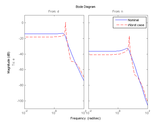
This analysis reveals that the nominal disturbance rejection properties of the controller C are not robust to the specified level of uncertainty.