This demo illustrates the application of robust control design (using D-K iteration) and robustness analysis to a process control problem. The plant is a simple two-tank system at Caltech. Other experimental work relating to this system is described by Smith et al. in the following references
The plant consists of two water tanks in cascade and is shown schematically in Figure 1. The upper tank (tank 1) is fed by hot and cold water via computer-controlled valves. The lower tank (tank 2) is fed by water from an exit at the bottom of tank 1. A constant level is maintained in tank 2 by means of an overflow. A cold water bias stream also feeds tank 2 and enables the tanks to have different steady-state temperatures.
The design objective is to control the temperatures of both tanks 1 and 2. The controller has access to the reference commands and the temperature measurements.
twotankpic = imread('twotank.jpg');
image(twotankpic); axis off image
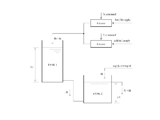
Figure 1. Schematic Diagram of the Two Tank System
The plant variables are given the following designations:
For convenience we define a system of normalized units as follows:
Variable Unit Name 0 means: 1 means:
temperature      tunit      cold water temp.    hot water temp.
height           hunit      tank empty          tank full
flow             funit      zero input flow     max. input flow
Using the above units, the plant parameters are:
A1 = 0.0256;	% area of tank 1 (hunits^2)
A2 = 0.0477;	% area of tank 2 (hunits^2)
h2 = 0.241;	   % height of tank 2, fixed by overflow (hunits)
fb = 3.28e-5;  % bias stream flow (hunits^3/sec)
fs = 0.00028;	% flow scaling (hunits^3/sec/funit)
th = 1.0;	   % hot water supply temp (tunits)
tc = 0.0;	   % cold water supply temp (tunits)
tb = tc;	      % cold bias stream temp (tunits)
alpha = 4876;  % constant for flow/height relation (hunits/funits)
beta = 0.59;   % constant for flow/height relation (hunits)
The variable fs is a flow scaling factor which converts the input (0 to 1 funits) to flow in hunits^3/second. The constants alpha and beta describe the flow/height relationship for tank 1: h1 = alpha*f1-beta.
The nominal tank models are obtained by linearizing around the following operating point (all normalized values):
h1ss = 0.75;                            % water level for tank 1
t1ss = 0.75;                            % temperature of tank 1
f1ss = (h1ss+beta)/alpha;               % flow tank 1 -> tank 2
fss = [th,tc;1,1]\[t1ss*f1ss;f1ss];
fhss = fss(1);                          % hot flow
fcss = fss(2);                          % cold flow
t2ss = (f1ss*t1ss + fb*tb)/(f1ss + fb); % temperature of tank 2
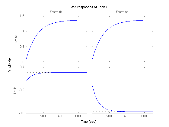
The nominal model for tank 1 has inputs [fh; fc] and outputs [h1; t1]
A = [ -1/(A1*alpha),          0;
      (beta*t1ss)/(A1*h1ss),  -(h1ss+beta)/(alpha*A1*h1ss)];

B = fs*[ 1/(A1*alpha),   1/(A1*alpha);
         th/A1,          tc/A1];

C = [ alpha,             0;
      -alpha*t1ss/h1ss,  1/h1ss];

D = zeros(2,2);
tank1nom = ss(A,B,C,D,'InputName',{'fh','fc'},'OutputName',{'h1','t1'});

clf
step(tank1nom), title('Step responses of Tank 1')
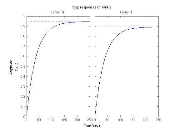
The nominal model for tank 2 has inputs [h1;t1] and output t2.
A = -(h1ss + beta + alpha*fb)/(A2*h2*alpha);
B = [ (t2ss+t1ss)/(alpha*A2*h2),  (h1ss + beta)/(alpha*A2*h2) ];
C = 1;
D = zeros(1,2);

tank2nom = ss(A,B,C,D,'InputName',{'h1','t1'},'OutputName','t2');

step(tank2nom), title('Step responses of Tank 2')
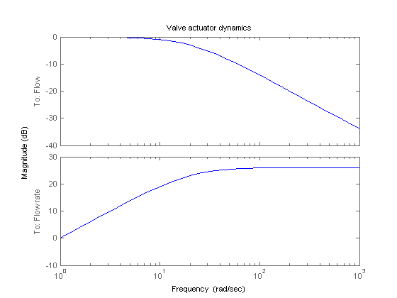
There are significant dynamics and saturations associated with the actuators so it is important to include actuator models. In the frequency range of interest, the actuators can be modeled as a first order system with rate and magnitude saturations. It is the rate limit, rather than the pole location, that limits the actuator performance for most signals. For a linear model some of the effects of rate limiting can be included in a perturbation model.
We initially set up the actuator model with one input (the command signal) and two outputs (the actuated signal and its derivative). The derivative output will be useful in limiting the actuation rate when designing the control law.
act_BW = 20;		% actuator bandwidth (rad/sec)
actuator = [ tf(act_BW,[1 act_BW]); tf([act_BW 0],[1 act_BW]) ];
actuator.OutputName = {'Flow','Flow rate'};

bodemag(actuator)
title('Valve actuator dynamics')

hot_act = actuator;
set(hot_act,'InputName','fhc','OutputName',{'fh','fh_rate'});
cold_act =actuator;
set(cold_act,'InputName','fcc','OutputName',{'fc','fc_rate'});
All measured signals are filtered with fourth-order Butterworth filters, each with a cutoff frequency of 2.25 Hz.
fbw = 2.25;		% antialiasing filter cut-off (Hz)
filter = mkfilter(fbw,4,'Butterw');
h1F = filter;
t1F = filter;
t2F = filter;
Open-loop experiments reveal some variability in the system responses and suggest that the linear models are only good at low frequency. If you fail to take this information into account during the design, your controller might perform poorly on the real system. This motivates building an uncertainty model that matches your estimate of uncertainty in the physical system as closely as possible. Because the amount of model uncertainty or variability typically depends on frequency, this uncertainty model involves frequency-dependent weighting functions to normalize modeling errors accross frequency.
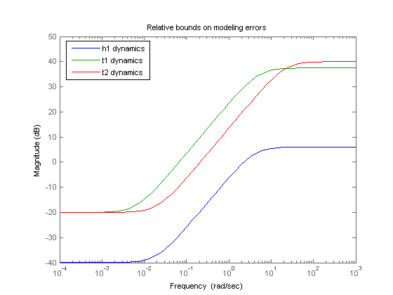
For example, open-loop experiments indicate that there is a significant amount of dynamic uncertainty in the t1 response. This is due primarily to mixing and heat loss. This can be modeled as a multiplicative (relative) model error Delta2 at the t1 output. Similarly, multiplicative model errors Delta1 and Delta3 can be added to the h1 and t2 outputs as shown in Figure 2.
clf
twotankuncpic = imread('twotankunc.jpg');
image(twotankuncpic); axis off image
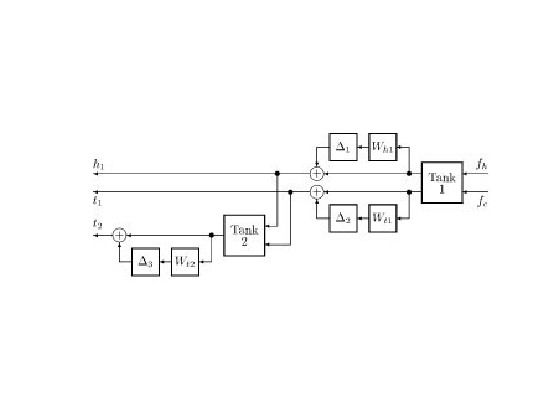
Figure 2. Schematic Representation of the Perturbed, Linear Two Tank System
To complete the uncertainty model, you must quantify how big the modeling errors are as a function of frequency. While it is difficult to precisely determine the amount of uncertainty in a system, you can look for rough bounds based on the frequency ranges where the linear model is accurate/poor. Here:
This data suggests the following choices for the frequency-dependent modeling error bounds.
Wh1 = 0.01+tf([0.5,0],[0.25,1]);
Wt1 = 0.1+tf([20*h1ss,0],[0.2,1]);
Wt2 = 0.1+tf([100,0],[1,21]);

clf
bodemag(Wh1,Wt1,Wt2), title('Relative bounds on modeling errors')
legend('h1 dynamics','t1 dynamics','t2 dynamics','Location','NorthWest')
You are now ready to build uncertain tank models that capture the modeling errors discussed above.
% Normalized error dynamics
delta1 = ultidyn('delta1',[1 1]);
delta2 = ultidyn('delta2',[1 1]);
delta3 = ultidyn('delta3',[1 1]);

% Frequency-dependent variability in h1, t1, t2 dynamics
varh1 = 1+delta1*Wh1;
vart1 = 1+delta2*Wt1;
vart2 = 1+delta3*Wt2;

% Add variability to nominal models
tank1u = append(varh1,vart1)*tank1nom;
tank2u = vart2*tank2nom;

tank1and2u = [eye(2); tank2u]*tank1u;
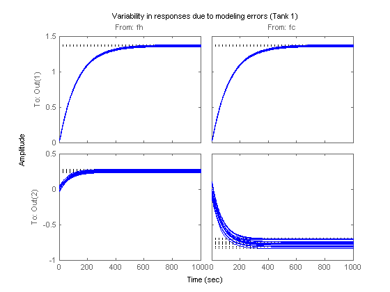
Randomly sample the uncertainty to see how the modeling errors might affect the tank responses
step(tank1u,1000), title('Variability in responses due to modeling errors (Tank 1)')
Let's now look at the control design problem. As mentioned above, you are interested in tracking setpoint commands for t1 and t2. To take advantage of H-infinity design algorithms, you must formulate your design as a closed-loop gain minimization problem. As usual, this is done by selecting weighting functions that capture the disturbance characteristics and performance requirements and help normalize the corresponding frequency-dependent gain constraints.
For the two-tank problem, a suitable weighted open-loop transfer function is shown below:
twotankicdesignpic = imread('twotankicdesign.jpg');
image(twotankicdesignpic);axis off image
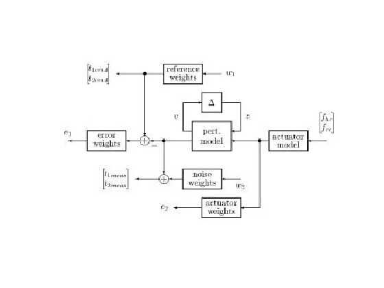
Figure 3. Control Design Interconnection for Two Tank System
You must now select weights for the sensor noises, setpoint commands, tracking errors, and hot/cold actuators.
The sensor dynamics are insignificant relative to the dynamics of the rest of the system. This is not true of the sensor noise. The potential sources of noise include electronic noise in thermocouple compensators, amplifiers, and filters, radiated noise from the stirrers, and poor grounding. Smoothed FFT analysis is used to estimate the noise level and suggests the following weights:
Wh1noise = 0.01;  % h1 noise weight
Wt1noise = 0.03;  % t1 noise weight
Wt2noise = 0.03;  % t2 noise weight
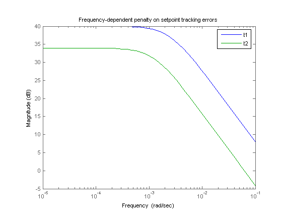
The error weights penalize setpoint tracking errors on t1 and t2. Pick first-order low-pass filters for these weights. You should use a higher weight (better tracking) for t1 because physical considerations lead to believe that t1 is easier to control than t2.
Wt1perf = tf(100,[400,1]);	% t1 tracking error weight
Wt2perf = tf(50,[800,1]);	% t2 tracking error weight

clf
bodemag(Wt1perf,Wt2perf)
title('Frequency-dependent penalty on setpoint tracking errors')
legend('t1','t2')
The reference (setpoint) weights reflect the frequency contents of such commands. Because the majority of the water flowing into tank 2 comes from tank 1, changes in t2 are dominated by changes in t1, and t2 is normally commanded to a value close to t1. So it makes more sense to use setpoint weighting expressed in terms of t1 and t2-t1:
t1cmd = Wt1cmd * w1
t2cmd = Wt1cmd * w1 + Wtdiffcmd * w2
where w1, w2 are white noise inputs. Adequate weight choices are:
Wt1cmd = 0.1;               % t1 input command weight
Wtdiffcmd = 0.01;           % t2 - t1  input command weight
Finally, we would like to penalize both the amplitude and the rate of the actuator. This can be done by weighting fhc (and fcc) with a function that rolls up at high frequencies. Alternatively, you can create an actuator model with fh and d|fh|/dt as outputs, and weight each output separately with constant weights. This approach has the advantage of reducing the number of states in the weigthed open-loop model.
Whact =  0.01;  % hot actuator penalty
Wcact =  0.01;  % cold actuator penalty

Whrate = 50;    % hot actuator rate penalty
Wcrate = 50;    % cold actuator rate penalty
Now that you have modeled all plant components and selected your design weights, you can use sysic to build an uncertain model of the weighted open-loop model shown in Figure 3.
systemnames = 'tank1and2u hot_act cold_act t1F t2F';
systemnames = [systemnames,' Wt1cmd Wtdiffcmd Whact Wcact'];
systemnames = [systemnames,' Whrate Wcrate'];
systemnames = [systemnames,' Wt1perf Wt2perf Wt1noise Wt2noise'];
inputvar = '[t1cmd;tdiffcmd;t1noise;t2noise;fhc;fcc]';
outputvar = '[Wt1perf;Wt2perf;Whact;Wcact;Whrate;Wcrate';
outputvar = [outputvar,'; Wt1cmd; Wt1cmd+Wtdiffcmd;'];
outputvar = [outputvar,' Wt1noise+t1F;  Wt2noise+t2F]'];
input_to_tank1and2u = '[hot_act(1);cold_act(1)]';
input_to_hot_act = '[fhc]';
input_to_cold_act = '[fcc]';
input_to_t1F = '[tank1and2u(2)]';
input_to_t2F = '[tank1and2u(3)]';
input_to_Wt1cmd = '[t1cmd]';
input_to_Wtdiffcmd = '[tdiffcmd]';
input_to_Whact = '[hot_act(1)]';
input_to_Wcact = '[cold_act(1)]';
input_to_Whrate = '[hot_act(2)]';
input_to_Wcrate = '[cold_act(2)]';
input_to_Wt1perf = '[Wt1cmd - tank1and2u(2)]';
input_to_Wt2perf = '[Wtdiffcmd + Wt1cmd - tank1and2u(3)]';
input_to_Wt1noise = '[t1noise]';
input_to_Wt2noise = '[t2noise]';
sysoutname = 'P';
cleanupsysic = 'yes';
echo off;sysic;echo on

disp('Weighted open-loop model: ')
P
Weighted open-loop model:
USS: 18 States, 10 Outputs, 6 Inputs, Continuous System
  delta1: 1x1 LTI, max. gain = 1, 1 occurrence
  delta2: 1x1 LTI, max. gain = 1, 1 occurrence
  delta3: 1x1 LTI, max. gain = 1, 1 occurrence
By construction of the weights and weighted open loop of Figure 3, you have recast your control problem as a closed-loop gain minimization. You can now easily compute a gain-minimizing control law for the nominal tank models:
nmeas = 4;		% number of measurements
nctrls = 2;		% number of controls
[k0,g0,gamma0] = hinfsyn(P.NominalValue,nmeas,nctrls);
gamma0
gamma0 =
    0.9024
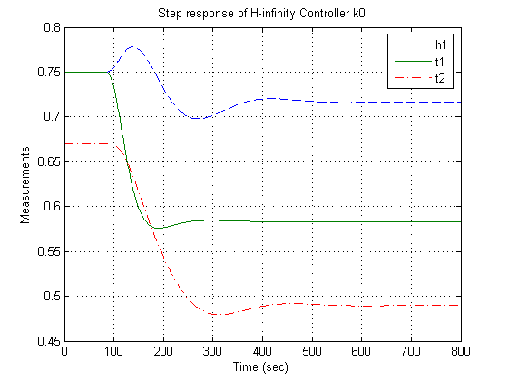
The smallest achievable closed-loop gain is about 0.9, which indicates that your frequency-domain tracking performance specifications are met by the controller k0. Simulating this design in the time domain is a reasonable way of checking that you have correctly set the performance weights. First create a closed-loop model mapping the input signals [ t1ref; t2ref; t1noise; t2noise] to the output signals [h1; t1; t2; fhc; fcc].
systemnames = 'tank1nom tank2nom hot_act cold_act t1F t2F';
inputvar = '[t1ref; t2ref; t1noise; t2noise; fhc; fcc]';
outputvar = '[ tank1nom; tank2nom; fhc; fcc; t1ref; t2ref; ';
outputvar = [outputvar 't1F+t1noise; t2F+t2noise]'];
input_to_tank1nom = '[hot_act(1); cold_act(1)]';
input_to_tank2nom = '[tank1nom]';
input_to_hot_act = '[fhc]';
input_to_cold_act = '[fcc]';
input_to_t1F = '[tank1nom(2)]';
input_to_t2F = '[tank2nom]';
sysoutname = 'simlft';
cleanupsysic = 'yes';
sysic;

% Close the loop with the H-infinity controller |k0|
sim_k0 = lft(simlft,k0);
sim_k0.InputNames = {'t1ref'; 't2ref'; 't1noise'; 't2noise'};
sim_k0.OutputNames = {'h1'; 't1'; 't2'; 'fhc'; 'fcc'};
Simulate the closed-loop response when ramping down the setpoints for t1 and t2 between 80 seconds and 100 seconds.
time=0:800;
t1ref = (time>=80 & time<100).*(time-80)*-0.18/20 + ...
    (time>=100)*-0.18;
t2ref = (time>=80 & time<100).*(time-80)*-0.2/20 + ...
    (time>=100)*-0.2;
t1noise = Wt1noise * randn(size(time));
t2noise = Wt2noise * randn(size(time));

y = lsim(sim_k0,[t1ref ; t2ref ; t1noise ; t2noise],time);
Add the simulated outputs to their steady state values and plot the responses.
h1 = h1ss+y(:,1);
t1 = t1ss+y(:,2);
t2 = t2ss+y(:,3);
fhc = fhss/fs+y(:,4); % note scaling to actuator
fcc = fcss/fs+y(:,5); % limits (0<= fhc <= 1) etc.
Plot the outputs, t1 and t2, as well as the height h1 of tank 1.
plot(time,h1,'--',time,t1,'-',time,t2,'-.');
xlabel('Time (sec)')
ylabel('Measurements')
title('Step response of H-infinity Controller k0')
legend('h1','t1','t2');
grid
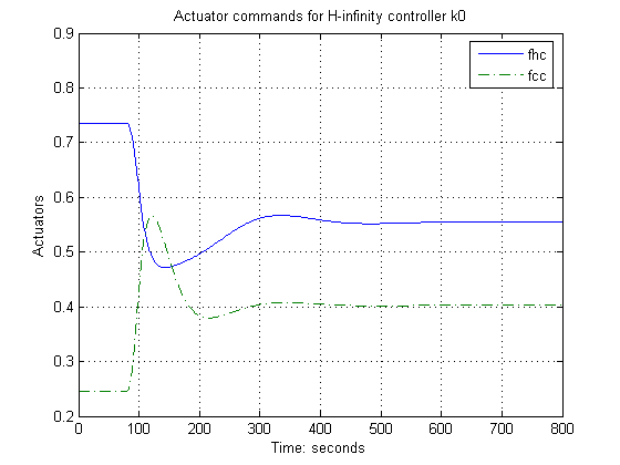
Plot the commands to the hot and cold actuators.
plot(time,fhc,'-',time,fcc,'-.');
xlabel('Time: seconds')
ylabel('Actuators')
title('Actuator commands for H-infinity controller k0')
legend('fhc','fcc');
grid
The H-infinity controller k0 was designed for the nominal tank models. How well does it fare for perturbed model within the model uncertainty bounds (see "Uncertainty on Model Dynamics")?
To answer this question, compare the nominal closed-loop performance gamma0 with the worst-case performance over the model uncertainty set
frad = 2*pi*logspace(-5,1,30);
clpk0 = lft(P,k0);
clpk0_g = frd(clpk0,frad);

% Compute worst-case gain
opt=wcgopt('FreqPtWise',1);
[maxgain,wcu,info] = wcgain(clpk0_g,opt);

% Compare closed-loop gains
clf
semilogx(fnorm(clpk0_g.NominalValue),'b-',...
   maxgain.UpperBound,'r--')
title('Performance analysis for controller k0')
xlabel('Frequency (rad/sec)')
legend('Nominal','Worst-case')
axis([1e-4 100 0 2.5])
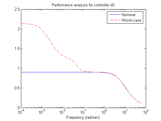
The worst-case performance of the closed-loop is significantly worse than the nominal performance so the H-infinity controller k0 is not robust to modeling errors.
To remedy this lack of robustness, you can use dksyn to design a controller that takes into account modeling uncertainty and delivers consistent performance for the nominal and perturbed models.
% Options for D-K iterations
opt = dkitopt('FrequencyVector',frad,'NumberofAutoIterations',4);

% Perform mu synthesis
[kmu,clpmu,bnd] = dksyn(P,nmeas,nctrls,opt);
bnd
Warning: Solution may be inaccurate due to poor scaling or eigenvalues near the stability boundary.
bnd =
    1.5221
As before, simulate the closed-loop responses with kmu
sim_kmu = lft(simlft,kmu);
y = lsim(sim_kmu,[t1ref;t2ref;t1noise;t2noise],time);
h1 = h1ss+y(:,1);
t1 = t1ss+y(:,2);
t2 = t2ss+y(:,3);
fhc = fhss/fs+y(:,4); % note scaling to actuator
fcc = fcss/fs+y(:,5); % limits (0<= fhc <= 1) etc.

% Plot |t1| and |t2| as well as the height |h1| of tank 1
plot(time,h1,'--',time,t1,'-',time,t2,'-.');
xlabel('Time: seconds')
ylabel('Measurements')
title('Step response of mu controller kmu')
legend('h1','t1','t2');
grid
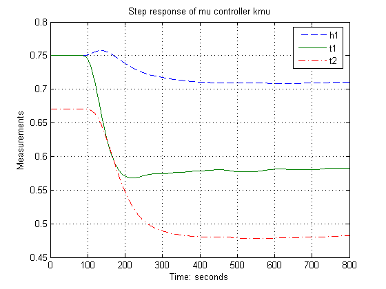
The time responses are comparable with those for k0 and show only a slight performance degradation. However, kmu fares better regarding robustness to unmodeled dynamics.
% Worst-case performance for kmu
clpmu_g = frd(clpmu,frad);
opt = wcgopt('FreqPtWise',1,'Sensitivity','On');
[maxgain,wcu,wcinfo] = wcgain(clpmu_g,opt);

% Compare closed-loop gains
clf
semilogx(fnorm(clpmu_g.NominalValue),'b',...
   maxgain.UpperBound,'r--')
title('Performance analysis for controller kmu')
xlabel('Frequency (rad/sec)')
legend('Nominal','Worst-case')
axis([1e-4 100 0 2.5])

% [perfmarg,wcu,report,rpinfo] = robustperf(clpmu_g);
% semilogx(rpinfo.MussvBnds(1),'b-.');
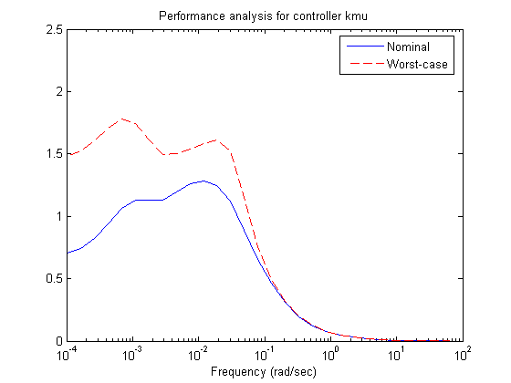
wcgain also returns local sensitivities of the worst-case gain to the variability of each uncertain element. The sensitivities imply that the peak on the worst-case gain curve is most sensitive to changes in the range of delta2.
idx = find(maxgain.CriticalFrequency==info.Frequency);
wcinfo.Sensitivity{idx}
ans =
    delta1: 0.0772
    delta2: 38.1081
    delta3: 5.9261