This demonstrates how to build uncertain state-space models and analyze the robustness of feedback control systems with uncertain elements.
You will learn how to specify uncertain physical parameters and create uncertain state-space models from these parameters. You will see how to evaluate the effects of random and worst-case parameter variations using the functions usample and robuststab.
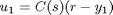
For this demo we use the following system consisting of two frictionless carts connected by a spring k
    % Display image file cartpic.png
    [fig1,mono]=imread('cartspic','png');image(fig1);
    axis off equal; colormap(mono);
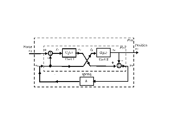
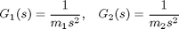
The control input is the force u1 applied to the left cart, and the output to be controlled is the position y1 of the right cart. The feedback control is of the form
and we use a triple-lead compensator

You can create this compensator by
    s = zpk('s'); % the Laplace 's' variable
    C = 100*ss((s+1)/(.001*s+1))^3;
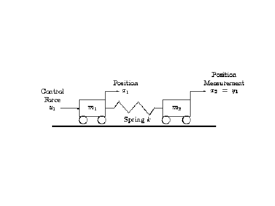
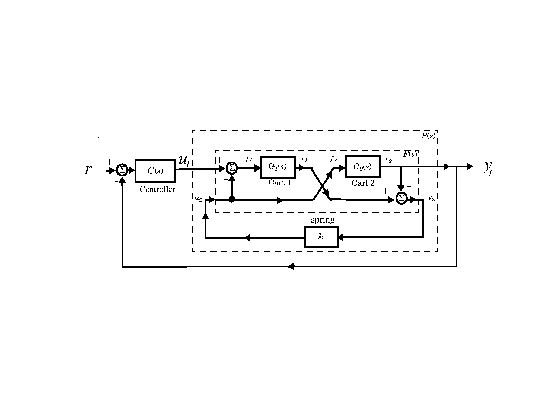
The two-cart and spring system is modeled by the block diagram shown below.
    % Display image file cartslft.png
    [fig2,mono]=imread('cartslft','png');image(fig2);
    axis off equal; colormap(mono);
The problem of controlling the carts is complicated by the fact that the values of the spring constant k and cart masses m1,m2 are known with only 20% accuracy: k=1.0±20%, m1=1.0±20% and m2=1.0±20%. To capture this variability, create three uncertain real parameters using ureal:
    k = ureal('k',1,'percent',20);
    m1 = ureal('m1',1,'percent',20);
    m2 = ureal('m2',1,'percent',20);
The carts models are
Given the uncertain parameters m1 and m2, you can construct uncertain state-space models (USS) for G1 and G2 as follows:
    G1 = 1/s^2/m1
    G2 = 1/s^2/m2
USS: 2 States, 1 Output, 1 Input, Continuous System
  m1: real, nominal = 1, variability = [-20  20]%, 1 occurrence
USS: 2 States, 1 Output, 1 Input, Continuous System
  m2: real, nominal = 1, variability = [-20  20]%, 1 occurrence
First construct a plant model P corresponding to the block diagram shown above (P maps u1 to y1):
    % Spring-less inner block F(s)
    F = [0;G1]*[1 -1]+[1;-1]*[0,G2];

    % Connect with the spring k
    P = lft(F,k);
The feedback control u1 = C*(r-y1) operates on the plant P as shown below:
    % Display image file cartsfeedback.png
    [fig3,mono]=imread('cartsfeedback','png');image(fig3);
    axis off equal; colormap(mono);
Use feedback to compute the closed-loop transfer from r to y1.
    % Uncertain open-loop model is
    L = P*C;

    % Uncertain closed-loop transfer from r to y1 is
    T = feedback(L,1)
USS: 7 States, 1 Output, 1 Input, Continuous System
   k: real, nominal = 1, variability = [-20  20]%, 1 occurrence
  m1: real, nominal = 1, variability = [-20  20]%, 1 occurrence
  m2: real, nominal = 1, variability = [-20  20]%, 1 occurrence
Note that since G1 and G2 are uncertain, both P and T are uncertain state-space models.
The nominal transfer function of the plant is
Pnom = zpk(P.nominal)
Zero/pole/gain:
      1
--------------
s^2 (s^2  + 2)
You can evaluate the nominal closed-loop transfer function Tnom, then check that all the poles of the nominal system have negative real parts:
    Tnom = zpk(T.nominal);
    maxrealpole = max(real(pole(Tnom)))
maxrealpole =
   -0.8232
Will the feedback loop remain stable for all possible values of k,m1,m2 in the specified uncertainty range? You can use the robuststab command to rigorously answer this question. robuststab computes the stability margins and the smallest destabilizing parameter variations Udestab (relative to the nominal values):
    [StabilityMargin,Udestab,REPORT] = robuststab(T);
    REPORT
    Udestab
REPORT =
Uncertain System is robustly stable to modeled uncertainty.
 -- It can tolerate up to 311% of modeled uncertainty.
 -- A destabilizing combination of 500% the modeled uncertainty exists,
    causing an instability at 79.3 rad/s.
 -- Sensitivity with respect to uncertain element ...
   'k' is 25%.  Increasing 'k' by 25% leads to a 6% decrease in the margin.
   'm1' is 59%.  Increasing 'm1' by 25% leads to a 15% decrease in the margin.
   'm2' is 55%.  Increasing 'm2' by 25% leads to a 14% decrease in the margin.
Udestab =
     k: 8.0026e-005
    m1: 8.0026e-005
    m2: 1.9999
REPORT indicates that the closed loop can tolerate up to 3 times as much variability in k,m1,m2 before going unstable. It also provides useful information about the sensitivity of stability to each parameter. Note that the smallest destabilizing perturbation Udestab requires varying m2 by 100%, or 5 times the specified uncertainty.
The peak gain across frequency of the closed-loop transfer T is indicative of the level of overshoot in the closed-loop step response. The closer this gain is to one, the smaller the overshoot is.
Use wcgain to compute the worst-case gain PeakGain of T over the specified uncertainty range.
    [PeakGain,Uwc] = wcgain(T);
    PeakGain
PeakGain =
           LowerBound: 1.0471
           UpperBound: 1.0479
    CriticalFrequency: 7.7081
Substitute the worst-case parameter variation Uwc into T to compute the worst-case closed-loop transfer Twc.
Twc = usubs(T,Uwc); % Worst-case closed-loop transfer T
Finally, pick for random samples of the uncertain parameters and compare the corresponding closed-loop transfers with the worst-case transfer Twc.
    Trand = usample(T,4);         % 4 random samples of uncertain model T
    clf
    subplot(211), bodemag(Trand,'b',Twc,'r',{10 1000});  % plot Bode response
    subplot(212), step(Trand,'b',Twc,'r',0.2);           % plot step response
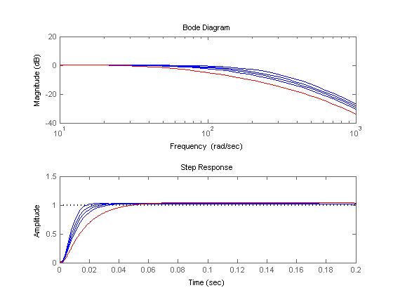
This analysis indicates the compensator C performs robustly for the specified uncertainty on k,m1,m2.
See also uss_demo.m