Analysis of Fixed-Point Numerically Controlled Oscillator

Contents

Introduction

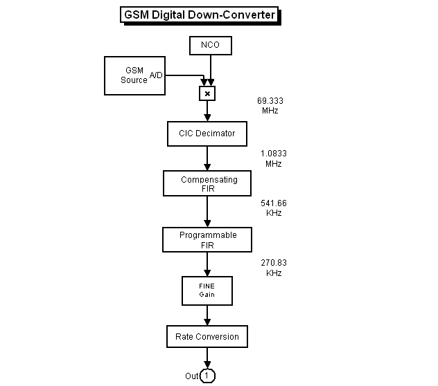
Digital Down-Converters (DDC) are a key component of digital radios. The DDC performs the frequency translation necessary to convert the high input sample rates found in a digital radio, down to lower sample rates (baseband) for further and easier processing. Adhering to the GSM specifications, in this example, the DDC's input rate is at 69.333 MHz and it is tasked with downconverting its input rate down to 270 KHz.

The DDC consists of a Numerically Controlled Oscillator (NCO) and a mixer to quadrature down convert the input signal to baseband. The baseband signal is then low pass filtered by a Cascaded Integrator-Comb (CIC) filter followed by two FIR decimating filters to achieve the desired low sample-rate ready for further processing. The final stage often includes a resampler which interpolates or decimates the signal to achieve the desired sample rate depending on the application. Further filtering can be achieved with the resampler. A block diagram of a typical DDC is shown below. One thing to note is that Simulink handles complex signals, so we don't have to treat the I and Q channels separately.

This demo focuses on the analysis of the NCO. For a demo on designing the three-stage, multirate, fixed-point filter chain and HDL code generation refer to the following demo Implementing the Filter Chain of a Digital Down-Converter in HDL.

The Numerically Controlled Oscillator (NCO)

The digital mixer section of the DDC includes a multiplier and a NCO, which provide channel selection or tuning for the radio. It is basically a sine and cosine generator, creating complex values for each sine/cosine pair. A typical NCO consists of four components, the phase accumulator, the phase adder, the dither generator, and sine/cosine lookup table.

Here's a typical NCO circuit modeled in Simulink, similar to what you would see in Graychip's data sheet.

open_system('ddcnco');

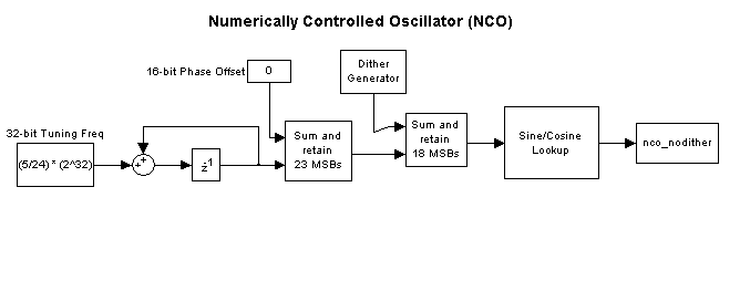
Based on the input frequency the NCO's phase accumulator produces values which are used to address a sine/cosine table lookup. The phase adder is used to specify a phase offset which provides the ability to phase modulate the output of the phase accumulator. Phase dithering is provided by the Dither Generator to reduce amplitude quantization noise and therefore improve the Spurious Free Dynamic Range of the NCO. The sine/cosine lookup table produces the actual complex sinusoidal signal and the output is stored in the variable nco_nodither.

In the Graychip the tuning frequency is specified as a normalized value relative to the chip's clock rate. So, for a tuning frequency of F the normalized frequency is F/Fck, where Fck is the chip's clock rate. The phase offset is specified in radians ranging between 0 and 2pi. In this demo the normalized tuning frequency is set to 5/24 while the phase offset is set to 0. The tuning frequency is specified as a 32 bit word and the phase offset is specified as a 16 bit word.

Since the NCO is implemented using fixed-point arithmetic, it experiences undesirable amplitude quantization effects. These are numerical distortions due to finite wordlength effects. Basically, we have sinusoids being quantized giving rise to cumulative, deterministic, periodic errors in the time domain, which appear as line spectra (spurs) in the frequency domain. The amount of attenuation from the peak of the signal of interest to the highest spur is the Spurious Free Dynamic Range.

The Spurious Free Dynamic Range (SFDR) of the Graychip is 106dB, however the GSM spec requires that the SFDR be > 110dB. There are a couple of ways to improve the SFDR, we will explore the use of adding phase dither to the NCO.

The Graychip's NCO contains a phase dither generator which is basically a random integer generator, and is used to improve the purity of the oscillator output. Dithering causes the unintended periodicities of the quantization noise (leading to "spikes" in spectra, poor SFDR) to be "spread" across a broad spectrum, effectively reducing these undesired spectral peaks. Conservation of energy applies, however, the spreading effectively raises the overall noise floor. So it's good for SFDR, but only up to a certain point.

Let's run the NCO model and analyze its output in MATLAB's workspace. This model is not using dithering.

sim('ddcnco');
whos nco*

  Name               Size                           Bytes  Class

  nco_nodither       1x1x20545                     328720  double array (complex)

Grand total is 20545 elements using 328720 bytes

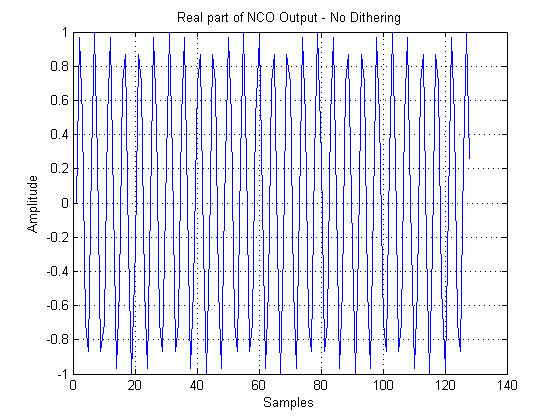
The plot below displays the real part of the first 128 samples of the output of the NCO, which is stored in the variable called nco_nodither.

plot(real(squeeze(nco_nodither(1:128)))); grid
title('Real part of NCO Output - No Dithering')
ylabel('Amplitude');
xlabel('Samples');
set(gcf,'color','white');

Spectral Analysis of NCO Output

When performing spectral estimation, it is very important to understand your data in order to choose the appropriate spectral estimation technique. Given that we have a large data set (over 20,000 samples), we can rely on an FFT based classical method, such as periodogram, to calculate the spectral content of the output of the NCO.

The signal has some randomness, however it's primarily sinusoidal, so we will measure its mean-square spectrum, as opposed to the power spectral density which is more appropriate to measure the power of random signals. For a demo on measuring power refer to Measuring the Power of Deterministic Periodic Signals. Below we use the msspectrum method to calculate and plot the Mean-square Spectrum of the NCO signal.

Define spectral analysis algorithm.

h = spectrum.periodogram

 
h =
 
    EstimationMethod: 'Periodogram'
           FFTLength: 'NextPow2'
          WindowName: 'Rectangular'

Calculate and plot the Mean-square Spectrum.

Fs = 69.333e6;
msspectrum(h,real(nco_nodither),'Fs',Fs)
set(gcf,'color','white');

Warning: Log of zero.

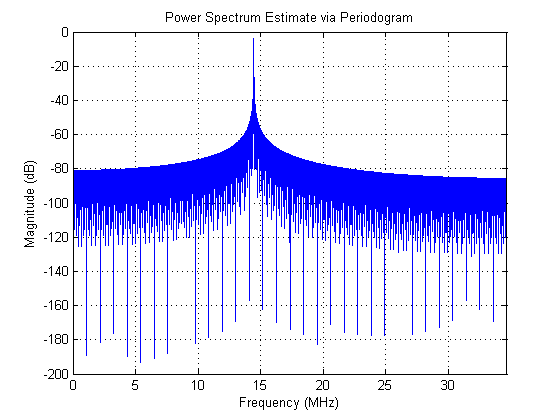
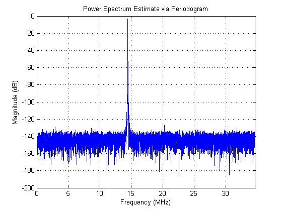
As expected, the Mean-square Spectrum plot shows a peak at 14.44 MHz, which is the NCO's tuning frequency 5/24*Fs = 14.444 MHz.

Notice however that the noise floor which is about -82 dB is too high to meet the GSM specifications, which requires -110 dB or more. We know we can improve this by adding phase dither, but before we add dither let's take a closer look at our analysis.

Choosing the right Window

The periodogram spectral analysis technique uses a rectangular window, which although it provides good frequency resolution (i.e., it has a narrow mainlobe bandwidth), it has a high noise floor. Multiplying the NCO signal which is sinusoidal, by a rectangular window is the same as convolving the two signals in the frequency domain. The convolution of a sinusoidal signal's frequency response, which is a delta, by a rectangular window, whose frequency response is a sin(x)/x, will result in a sin(x)/x response centered at the frequency of the delta. So, there's a smearing of the delta function in the frequency domain. The noise floor will be the addition of the two signals. Therefore, what we're seeing is the noise floor of the rectangular window, which is much higher than the highest signal spur.

To verify that the noise floor of the window is preventing us from seeing the signal spurs, let's look at the time and frequency response of rectangular window. We can design such a window using the Window Design Tool, WinTool, but here we will use the command line functionality.

Define and view the frequency response of a rectangular window.

N = length(nco_nodither);
wrect = sigwin.rectwin(N)

 
wrect =
 
      Name: 'Rectangular'
    Length: 20545

wvtool(wrect)

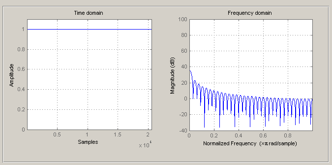
If we zoom in or use data markers we see that the maximum attenuation the rectangular window achieves is about 84 dB, which is roughly the noise floor we saw in the spectrum plot of the NCO output.

Since in our analysis we're not trying to resolve two sinusoids, but instead we're looking for spectral content below 100 dB, let's use a Von Hann window which provides over 100 dB of attenuation.

whann = sigwin.hann(N)

 
whann =
 
            Name: 'Hann'
          Length: 20545
    SamplingFlag: 'symmetric'

Let's view the Hann window both in time and frequency domain.

wvtool(whann)

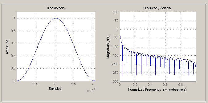
Indeed the frequency domain plot on the right shows that the Hann window exhibits a much lower noise floor. So, the Von Hann window is better suited for this particular problem. Here are the results of using the Hann window to calculate the spectral estimate of the NCO output.

h.WindowName = 'Hann';
msspectrum(h,real(nco_nodither),'Fs',Fs);
set(gcf,'color','white');

Warning: Log of zero.

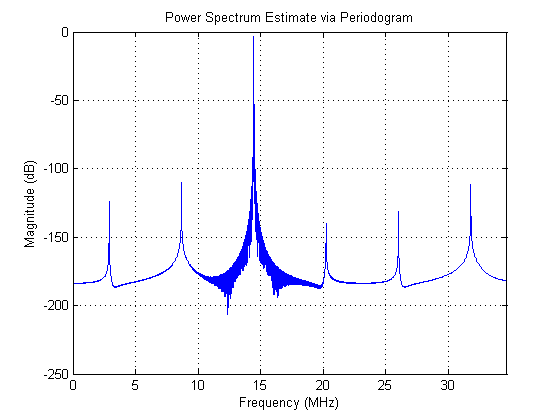
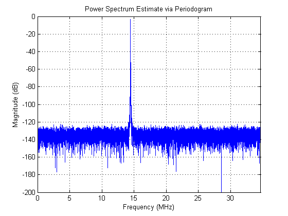
Using a Hann window to window our NCO signal produced a much lower noise floor clearly displaying the spurious peaks. Now we can measure the Spurious Free Dynamic Range (SFDR) and look into ways to decrease the spurious peaks by using phase dithering.

We can zoom-in using the axis command to measure the difference between the peak of the carrier and the highest spurious peak.

axis([0 35 -5 0])

The peak is roughly -3.25dB. Now let's zoom-in to the highest spur.

axis([0 35 -120 -100])

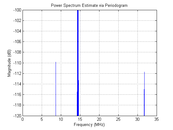
The highest spur is -110 dB. The Spurious Free Dynamic Range then is the difference between these two values 110dB - 3.25dB = 106.75 dB.

Exploring the Effects of Dithering

In order to explore the effects of adding dither to the NCO, I have encapsulated the NCO circuit shown above in a subsystem and duplicated the NCO subsystem three times. Then a different amount of dither was selected in each NCO. The NCO allows a range of 1 to 19 bits of dither to be specified, however we'll just try a few values. Running this model will produce three different NCO outputs based on the amount of dither added.

open_system('ddcncowithdither')

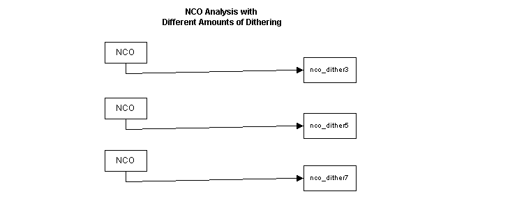
Running the simulation will produce three signals in the MATLAB workspace that we can then analyze using the same spectral analysis algorithm defined above. We can run the simulation from the model or from the command line using the sim command.

sim('ddcncowithdither')

After the simulation completes we're left with the signals which are the output of the NCOs with varying amounts of dithering.

whos nco*

  Name               Size                           Bytes  Class

  nco_dither3        1x1x20501                     328016  double array (complex)
  nco_dither5        1x1x20501                     328016  double array (complex)
  nco_dither7        1x1x20501                     328016  double array (complex)
  nco_nodither       1x1x20545                     328720  double array (complex)

Grand total is 82048 elements using 1312768 bytes

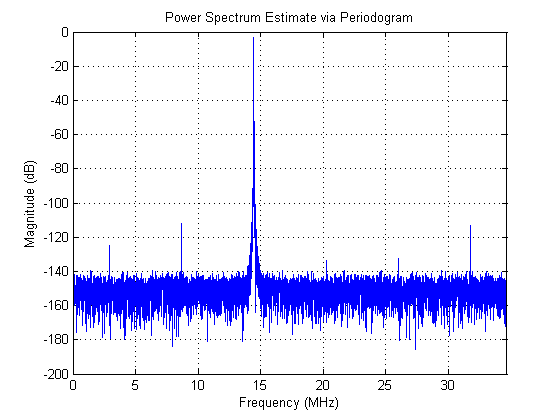
As already seen above, using a Von Hann window we can see the spurious peaks, and as expected, since we're modeling a Graychip, the highest spur is at about -110 dB. The Spurious Free Dynamic Range then is about 107 dB, but our GSM spec requires that it be at least 110 dB. This is where dithering will help.

Let's start by adding 3 bits of dithering.

msspectrum(h,real(nco_dither3),'Fs',Fs) % Plot Mean-square Spectrum
set(gcf,'color','white');

Warning: Log of zero.

Again, let's zoom-in using the axis command to measure the difference between the peak of the carrier and the highest spurious peak.

axis([0 35 -5 0])

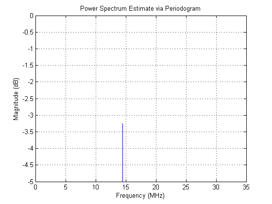
As expected the peak is again roughly -3.25 dB. Now let's zoom-in to the highest spur.

axis([0 35 -120 -100])

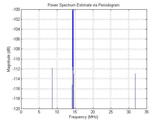
With three bits of dither added, the highest spur is now about 112 dB. The SFDR then is 112dB - 3.25dB = 108.75 dB. Still doesn't meet the GSM specification which requires an SFDR of 110 dB or more.

Let's try adding 5 bits of dithering.

msspectrum(h,real(nco_dither5),'Fs',Fs) % Plot Mean-square Spectrum
set(gcf,'color','white');

Warning: Log of zero.

The peak of the carrier frequency should still be roughly -3.25 dB. Now let's zoom-in to the highest spur.

axis([0 35 -130 -120])

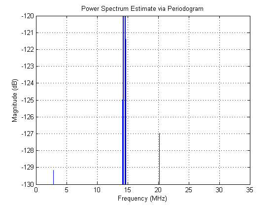
With five bits of dither added, the highest spur is now about -127 dB. The SFDR then is 127dB - 3.25dB = 123.75 dB. This SFDR meets and even exceeds the GSM specification.

So far the more dither we added the better the results were. So, let's try adding 7 bits of dithering.

msspectrum(h,real(nco_dither7),'Fs',Fs) % Plot Mean-square Spectrum
set(gcf,'color','white');

Warning: Log of zero.

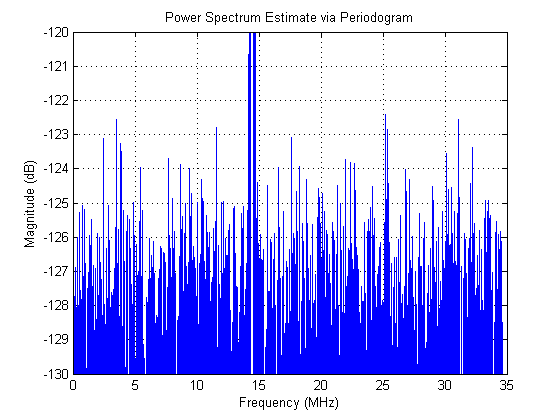
Zooming in on the noise floor we notice that highest spur is around -122.5 dB, which results in an SFDR of 119.25 dB. This meets the GSM spec, but we can do better using 5 bits of dithering.

axis([0 35 -130 -120])

Comparing Results

Let's tabulate the SFDR for each NCO output given the various amounts of dithering.

 Number of   Spur Free Dynamic
Dither bits   Range(dBc)

   0            107

   3            109

   5            123

   7            119

Summary

In this demo we analyzed the output of a Numerically Controlled Oscillator (NCO) used in a Digital Down Converter for a GSM application. We used spectral analysis to measure the Spurious Free Dynamic Range (SFDR), which is the difference between the highest spur and the peak of the signal of interest. Spurs are deterministic, periodic errors that result from quantization effects. We also explored the effects of adding dither in the NCO, which is a process that adds random data to the NCO to improve its purity. We found that using five bits of dithering achieved the highest SFDR.

Published with MATLAB® 7.0.2