Computational delays and sampling effects can critically effect the performance of a control system. Typically, the closed loop responses of a system will become oscillatory and unstable if these factors are not taken into account. Therefore when modeling a control system, computational delays and sampling effects should be included to accurately design and simulate a closed loop system.
There are two ways to approach the design of compensators with the effects of computational delay and sampling. The first approach is performed entirely in the discrete domain to capture the effects of sampling by discretizing the plant. The second approach is to to perform the design of a controller in the continuous domain which is sometimes more convenient, but in this case the effects of computational delay and sampling should be accounted for. In this demonstration, both approaches will be applied to redesign a control system using Simulink Control Design.
The following example model is of the speed control of a spark ignition engine. The initial compensator was designed on a linearized version of the continuous plant. See the Simulink Control Design demo on Extracting a Plant Model from a Simulink Model for Control Design for details.
First, specify the continuous feedback controller.
C = zpk(-2.89,0,0.0018222)
Zero/pole/gain:
0.0018222 (s+2.89)
------------------
        s
The first model is a discretized model, shown below.
mdl = 'scdspeed_compdelay';
open_system(mdl);
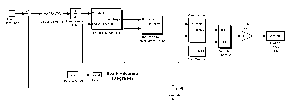
In this model the effects of the computational delay is modeled in the block scdspeed_compdelay/Compational Delay where the delay is equal to the worst case, the sample time of the controller. A zero order hold block scdspeed_compdelay/Zero-Order Hold is added to model the effects of sampling on the response of the system. Finally, the Speed Controller is descretized using a zero-order hold sampling method.
The effect of the sampling can be seen immediately by simulating the response of the system. The first sample time that is chosen is Ts = 0.1 seconds.
Ts = 0.1;
set_param('scdspeed_compdelay/Speed Controller','IC','286');
sim(mdl);
T2 = simout.time;
Y2 = simout.signals.values;
Next the sample time is increased to Ts = 0.25 seconds.
Ts = 0.25;
set_param('scdspeed_compdelay/Speed Controller','IC','181');
sim(mdl);
T3 = simout.time;
Y3 = simout.signals.values;
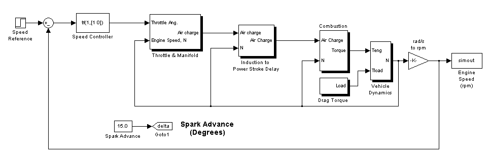
The second model is a continuous model, shown below
mdl_continuous = 'scdspeedctrl';
open_system(mdl_continuous);
To simulate the response of the continuous model the following commands are used.
set_param('scdspeedctrl/Speed Controller','sys','ss(C)');
set_param('scdspeedctrl/Speed Controller','IC','90.5581');
sim(mdl_continuous);
T1 = simout.time;
Y1 = simout.signals.values;
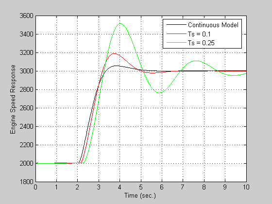
The plots of the responses are shown below. Note that the response becomes more oscillatory as the sample time is increased.
figure
plot(T1,Y1,'k')
hold on
plot(T2,Y2,'r')
plot(T3,Y3,'g')
xlabel('Time (sec.)')
ylabel('Engine Speed Response');
legend('Continuous Model','Ts = 0.1','Ts = 0.25');
grid
To remove the oscillatory effects of the closed loop system with the slowest sample time of Ts = 0.25 the compensator needs to be redesigned. A first appoach is to redesign using a discretized version of the plant. In this case the multirate model scdspeed_compdelay can be directly linearized.
Ts = 0.25;
Linearize the model
op = operpoint(mdl);
io(1) = linio('scdspeed_compdelay/Speed Controller',1,'in');
io(2) = linio('scdspeed_compdelay/Zero-Order Hold',1,'out','on');
sysd = linearize(mdl,op,io);
The linearized model for the sample time of 0.25 is redesigned by launching the SISO Tool.
sisotool(sysd,c2d(C,Ts))
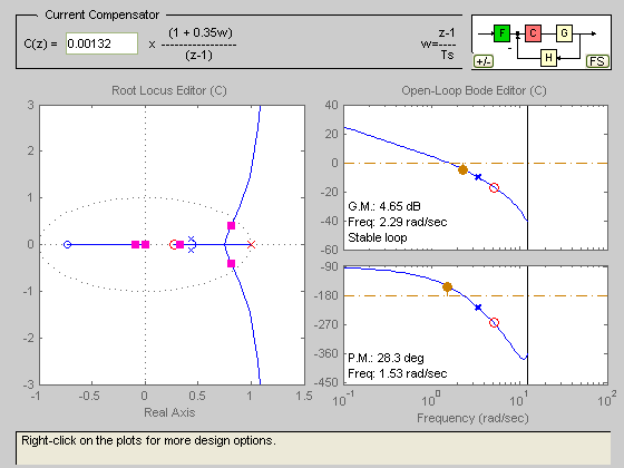
Using SISO Tool to redesign the controller gives the following controller.
Cd = zpk(0.2775,1,0.00066,Ts)
Zero/pole/gain:
0.00066 (z-0.2775)
------------------
      (z-1)

Sampling time: 0.25
This compensator then be used in the original model by setting the initial condition for the controller
set_param('scdspeed_compdelay/Speed Controller','sys','ss(Cd)');
set_param('scdspeed_compdelay/Speed Controller','IC','500');
Simulating the resulting closed loop system with a sample time Ts = 0.25. These results will be examined later.
sim(mdl);
Td = simout.time;
Yd = simout.signals.values;
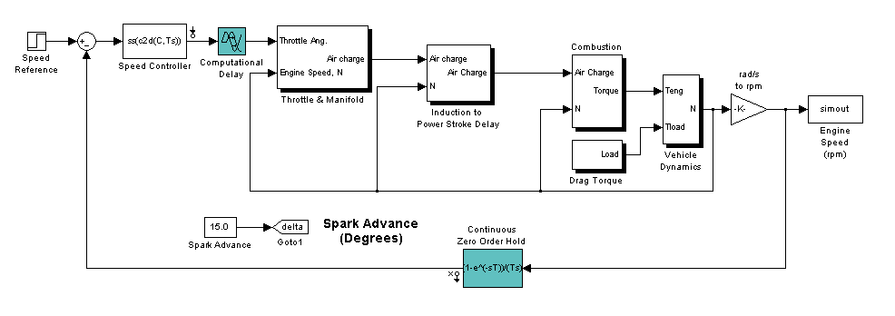
A second approach to redesigning the controller is to design with the continuous equivalents of the unit delay and zero order hold in place. The analysis of the controller design then remains in the continuous domain. The delay block, scdspeed_compdelay/Computational Delay is replaced with a continous transport delay. When linearizing the model a Pade approximation is used for the transport delay. Also, the zero order hold scdspeed_compdelay/Zero-Order Hold is replaced by its continuous representation.
The model with these replacements is shown below.
mdl_red = 'scdspeed_compdelay_remodeled';
open_system(mdl_red);
Now linearize the model with delays of Ts = 0.1 and 0.25.
op = operpoint(mdl_red);
io(1) = linio('scdspeed_compdelay_remodeled/Speed Controller',1,'in');
io(2) = linio('scdspeed_compdelay_remodeled/Continuous Zero Order Hold',1,'out','on');

Ts = 0.1;
sys2 = linearize(mdl_red,op,io);

Ts = 0.25;
sys3 = linearize(mdl_red,op,io);
Finally, the model without the effects of sampling and the computational delay is linearized using the commands below.
op = operpoint(mdl_continuous);
io(1) = linio('scdspeedctrl/Speed Controller',1,'in');
io(2) = linio('scdspeedctrl/rad//s to rpm',1,'out','on');
sys1 = linearize(mdl_continuous,op,io);
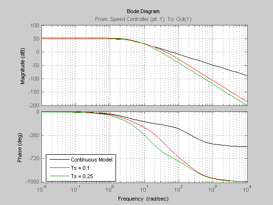
The linear models of the engine can be used to examine the effects of the computational delay on the frequency response. In this case the phase response of the system is significantly reduced due to the delay introduced by sampling.
figure
p = bodeoptions('cstprefs');
p.Grid = 'on';
p.PhaseMatching = 'on';
bodeplot(sys1,'k',sys2,'r',sys3,'g',p);
legend('Continuous Model','Ts = 0.1','Ts = 0.25','Location','SouthWest');
The linearized model for the slowest sample time is redesigned by launching the SISO Tool.
sisotool(sys3,C);
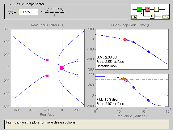
Using SISO Tool to redesign the controller gives the following controller.
Cc = zpk(-2.89,0,0.00066155)
Zero/pole/gain:
0.00066155 (s+2.89)
-------------------
         s
This compensator then be used in the original model by setting the initial condition for the controller.
set_param('scdspeed_compdelay/Speed Controller','sys','ss(c2d(Cc,Ts))');
set_param('scdspeed_compdelay/Speed Controller','IC','499');
Simulate the resulting closed loop system with a sample time Ts = 0.25.
sim(mdl);
Tc = simout.time;
Yc = simout.signals.values;
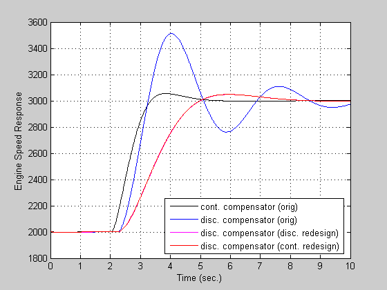
The plot below summarizes the responses of each design. The redesign of the control system using both approaches yields similar controllers. This example has displayed the effects of the computational delay and discretization. These effects reduce the stability margins of the system, but when a control system is properly modeled a desired closed loop behavior can be designed.
figure
plot(T1,Y1,'k',T3,Y3,'b',Td,Yd,'m',Tc,Yc,'r')
xlabel('Time (sec.)')
ylabel('Engine Speed Response');
h = legend('cont. compensator (orig)','disc. compensator (orig)', ...
    'disc. compensator (disc. redesign)',...
    'disc. compensator (cont. redesign)',...
    'Location','SouthEast');
grid