I = imread('peppers.png');
I = I(10+[1:256],222+[1:256],:);
figure;imshow(I);title('Original Image');
Deblurring Images Using the Wiener Filter
Wiener deconvolution can be used effectively when the frequency characteristics of the image and additive noise are known, to at least some degree.
| Key concepts: |
Deconvolution, image recovery, PSF, auto correlation functions |
| Key functions |
deconvwnr, imfilter, imadd |
Overview of Demo
The demo includes these steps:
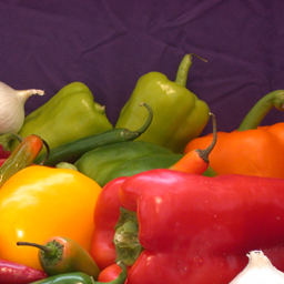
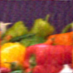
Step 1: Read in Images
The example reads in an RGB image and crops it to be 256-by-256-by-3. The deconvwnr function can handle arrays of any dimension.
I = imread('peppers.png');
I = I(10+[1:256],222+[1:256],:);
figure;imshow(I);title('Original Image');
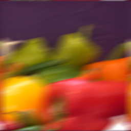
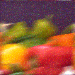
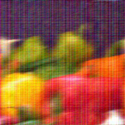
Step 2: Simulate a Motion Blur
Simulate a a real-life image that could be blurred e.g., by camera motion. The example creates a point-spread function, PSF, corresponding to the linear motion across 31 pixels (LEN=31), at an angle of 11 degrees (THETA=11). To simulate the blur, the filter is convolved with the image using imfilter.
LEN = 31;
THETA = 11;
PSF = fspecial('motion',LEN,THETA);
Blurred = imfilter(I,PSF,'circular','conv');
figure; imshow(Blurred);
title('Blurred');
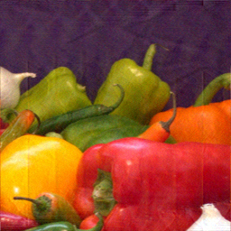
Step 3: Restore the Blurred Image
To illustrate the importance of knowing the true PSF in deblurring, this example performs three restorations. The first restoration, wnr1, uses the true PSF, created in Step 2.
wnr1 = deconvwnr(Blurred,PSF);
figure;imshow(wnr1);
title('Restored, True PSF');
The second restoration, wnr2, uses an estimated PSF that simulates motion twice as long as the blur length (LEN).
wnr2 = deconvwnr(Blurred,fspecial('motion',2*LEN,THETA));
figure;imshow(wnr2);
title('Restored, "Long" PSF');
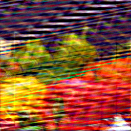
The third restoration, wnr3, uses an estimated PSF that simulates an angle of the motion twice as steep as the blur angle (THETA).
wnr3 = deconvwnr(Blurred,fspecial('motion',LEN,2*THETA));
figure;imshow(wnr3);
title('Restored, Steep');
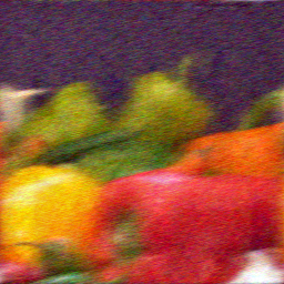
Step 4: Simulate Additive Noise
Simulate additive noise by using normally distributed random numbers and add it to the blurred image, Blurred, created in Step 2.
noise = 0.1*randn(size(I));
BlurredNoisy = imadd(Blurred,im2uint8(noise));
figure;imshow(BlurredNoisy);title('Blurred & Noisy');
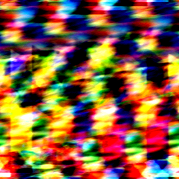
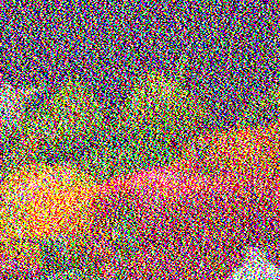
Step 5: Restore the Blurred and Noisy Image
Restore the blurred and noisy image using an inverse filter, assuming zero-noise, and compare this to the first result achieved in Step 3, wnr1. The noise present in the original data is amplified significantly.
wnr4 = deconvwnr(BlurredNoisy,PSF);
figure;imshow(wnr4);
title('Inverse Filtering of Noisy Data');
To control the noise amplification, provide the noise-to-signal power ratio, NSR.
NSR = sum(noise(:).^2)/sum(im2double(I(:)).^2);
wnr5 = deconvwnr(BlurredNoisy,PSF,NSR);
figure;imshow(wnr5);
title('Restored with NSR');
Vary the NSR value to affect the restoration results. The small NSR value amplifies noise.
wnr6 = deconvwnr(BlurredNoisy,PSF,NSR/2);
figure;imshow(wnr6);
title('Restored with NSR/2');
Step 6: Use Autocorrelation to Improve Image Restoration
To improve the restoration of the blurred and noisy images, supply the full autocorrelation function (ACF) for the noise, NCORR, and the signal, ICORR.
NP = abs(fftn(noise)).^2;
NPOW = sum(NP(:))/prod(size(noise)); % noise power
NCORR = fftshift(real(ifftn(NP))); % noise ACF, centered
IP = abs(fftn(im2double(I))).^2;
IPOW = sum(IP(:))/prod(size(I)); % original image power
ICORR = fftshift(real(ifftn(IP))); % image ACF, centered

wnr7 = deconvwnr(BlurredNoisy,PSF,NCORR,ICORR);
figure;imshow(wnr7);
title('Restored with ACF');
Explore the restoration given limited statistical information: the power of the noise, NPOW, and a 1-dimensional autocorrelation function of the true image, ICORR1.
ICORR1 = ICORR(:,ceil(size(I,1)/2));
wnr8 = deconvwnr(BlurredNoisy,PSF,NPOW,ICORR1);
figure;imshow(wnr8);
title('Restored with NP & 1D-ACF');