
Report of
RVIB Nathaniel B. Palmer Cruise 0202
to the
Western Antarctic Peninsula
9 April to 21 May, 2002
Report prepared by Peter Wiebe, John Klinck, Carin Ashjian, Erik Chapman, Wendy Kozlowski, Dezhang Chu, Rob Masserini, Deb Glasgow, Julian Ashford, Ana Sirovic, Phil Alatalo, Kristin Cobb, and Suzanne O’Hara, with assistance from other colleagues in the scientific party and the Raytheon Support Services. This cruise was sponsored by the Office of Polar Programs at the National Science Foundation.
United States Southern Ocean
Global Ocean Ecosystems Dynamics Program
Report Number 6
Available from
U.S. Southern Ocean GLOBEC Planning Office
Center for Coastal Physical Oceanography
Crittenton Hall
Old Dominion University
Norfolk, VA 23529
Acknowledgments
This cruise, the third in the series of four Southern Ocean GLOBEC broad-scale cruises, was in all measures a great success. The cruise objectives were accomplished as well or better than anticipated and there was time to add additional scientific activities to explore in greater depth some of the cruise findings. The Raytheon Marine Technical support group, led by Alice Doyle, provided excellent assistance in port and at sea. Their very positive attitude and superb technical expertise made the cruise run very smoothly. Captain Joe Borkowski and the officers and crew of the N.B. Palmer were also very supportive. The congenial atmosphere on board the N. B. Palmer made working and living there a great experience.
NBP0202 Cruise Participants on the RVIB N.B. Palmer
Kneeling (L-R): Alice Doyle, Jenny White, Phil Alatalo, John Klinck, Ann Sirovic, Amy Kukulya, Deb Glasgow, Helena Martellero, Wendy Kozlowski.
Row 1 (starting right of middle): Gaelin Rosenwaks, Yulia Serebrennikova, Kristy Aller, Andy Girard.
Row 2: Peter Wiebe, Carin Ashjian, Pete Martin, Karen Riener, Phil Taisey, Mark Dennett, Chris MacKay, Kristin Cobb, Erik Chapman, Steve Tarrent, Matthew Becker, Andres Hector Sepulveda, Romeo Laiviera, Sheldon Blackman, Tim Boyer, Rob Masserini, Julian Ashford, Dezhang Chu.
Row 3 (Upper right): Suzanne O’Hara, Kevin Bliss, Stian Alessandrini.
TABLE OF CONTENTS
1.0 Report for Hydrography, Circulation, and Meteorology Component
1.2 Details of Data Collection
1.2.5 Meteorology Measurements
1.3.1 Water Mass Distributions
1.3.2 Spatial Distributions and Circulation
2.4 Preliminary Results for Nutrient Concentrations
3.0 Primary Production Component
4.1 Zooplankton Sampling with the 1m2 MOCNESS Net System
4.2.1 Acoustics Data Collection, Processing, and Results
4.2.3.3.3 Video Recording and Processing
4.2.3.3.4 Plankton Abundance and Environmental Data
4.2.3.4.1 Planktonic Taxa Observed with the VPR
4.2.3.5.1 Plankton Distributions
4.2.4 Water column hydrographic and environmental characteristics
4.2.4.2 Distributional Patterns of Environmental Data
4.3 ROV observations of juvenile krill distribution, abundance, and behavior
5.0 Material Properties Of Zooplankton
5.2.1 Sound speed contrast measurements
5.2.2 Density contrast measurements
5.3 Data Collection and Preliminary Results
6.0 Seabird and Crabeater Seal Distribution in the Marguerite Bay Area
6.3.3.3 Adelie Penguin (Pygoscelis adeliae)
6.3.3.4 Crabeater Seals (Lobodon carcinophagus)
6.3.5.3 Data Collected/Preliminary Results
7.0 International Whaling Commission Cetacean Visual Survey
7.4 Preliminary findings/Discussion
8.0 Marine Mammals Passive Acoustics
11.0 Seabeam bathymetry of region and Mooring surveys
Appendix 2. Summary of CTD casts
Appendix 3. Summary of water samples
Appendix 4. Summary of salinity measurements
Appendix 5. Summary of oxygen titrations
Appendix 6. Summary of expendable probes
Appendix 7. Video and Lugol's Samples Taken on NBP0202
Appendix 8. Summary of sightings
Appendix 9. Results from analysis of fourteen diet samples of Adelie Penguins
Appendix 10. 1-m Ring Net Tow Information.
Appendix 11. BIOMAPER-II Tape Log.
Appendix 12. Cetacean Sightings NBP0202 9 April to 21 May 2002
The U.S. Southern Ocean GLOBEC Program is in its second field year. The focus of this study is on the biology and physics of a region of the continental shelf to the west of the Western Antarctic Peninsula extending from the northern tip of Adelaide Island to the southern portion of Alexander Island and including Marguerite Bay. The primary goals are:
1) To elucidate shelf circulation processes and their effect on sea ice formation and Antarctic krill (Euphausia superba) distribution.
2) To examine the factors that govern krill survivorship and availability to higher trophic levels, including seals, penguins, and whales.
The second year field program began with a mooring cruise in February and March aboard the R/V L.M. Gould during which a series of moorings deployed a year ago across the continental shelf of the Adelaide Island and across the mouth of Marguerite Bay were recovered (LMG02-1A Cruise Report). The Marguerite Bay moorings were reset in slightly different positions. In addition the series of bottom mounted moorings instrumented to record marine mammal calls and sounds were recovered and reset. This report describes and details the first broad-scale cruise to take place this year (the third in a series of four). Our effort is mainly devoted to developing a shelf-wide context for the process work being conducted during this same time period aboard the R/V L.M. Gould and for the modelers who will be using both the broad-scale and the process data in their model computations. Our specific objectives with regard to the broad-scale survey were:
1) To conduct a broad-scale survey of the SO GLOBEC Study Site to determine the abundance and distribution of the target species, Euphausia superba and its associated flora and fauna.
2) To conduct a hydrographic survey of the region.
3) To collect physical microstructure data from the water column.
4) To collect chlorophyll data, nutrient data, and to make primary production measurements to characterize the primary production of the region.
5) To collect zooplankton samples with a MOCNESS at selected locations throughout the broad-scale sampling area.
6) To survey the under ice distribution and abundance of krill larvae using an ROV equipped with a VPR, ADCP, and CTD.
7) To survey the sea birds throughout the broad-scale sampling area and determine their feeding patterns.
8) To survey the marine mammals throughout the broad-scale sampling area both by visual sightings and by passive listening techniques.
9) To map the bank-wide velocity field using an Acoustic Doppler Current Profiler (ADCP).
10) To collect acoustic, video, and environmental data along the tracklines between stations using a suite of sensors mounted in a towed body (BIOMAPER-II).
11) To collect meteorological data.
12) To deploy satellite tracked drogues at four locations on the station grid.
In addition, an ancillary program was conducted to study the sound speed contrast and the density contrast of zooplankton in the region, with principal focus on Antarctic krill.
The cruise track was determined by the positions of 92 station locations distributed along 13 transect lines running across the continental shelf and perpendicular to the Western Peninsula coastline (Figures 1, 2). The work was a combination of station and underway activities (See the Event Log, Appendix 1). The along-track data were collected from the BIo-Optical Multifrequency Acoustical and Physical Environmental Recorder (BIOMAPER-II), the ADCP, the meteorological sensors, through hull sea surface sensors, XBTs, XCTDs, and Sonabuoys. At the stations, a cast with a CTD/Rosette equipped with oxygen, transmissometer, and fluorometer sensors was made to the bottom. In water depths less than about 500 m, a Fast Repetition Response Fluorometer (FRRF) was added to the Rosette and at some deep water locations, a special cast to 100 m was made with it on before doing the deep cast. In addition, a sensor system to measure microstructure, CMiPS, was installed on the CTD and it was used on most CTD casts that were shallower than about 2000 m. At selected stations, a 1-m2 Multiple Opening/Closing Net and Environmental Sensing System (MOCNESS) was towed obliquely between the surface and near the bottom or 1000 m if the bottom were deeper for collection of zooplankton (335 um mesh). A 1-m Reeve net was used to make collections of live animals for use in shipboard acoustic experimental studies and a 1-m ring net was used for surface zooplankton collections for use in sea bird feeding studies. Meteorological, sea surface hydrographic properties, and SeaBeam bathymetry data were collected along the survey tracklines.
Note: all times given in the text are local times, which were +4 UTC time.
This narrative is an excerpt of reports usually sent in daily from the N.B. Palmer to the Southern Ocean GLOBEC Web Site located at: www.ccpo.odu.edu/Research/globec/main_cruises02/nbp0202/menu.html. These reports provide additional detail about the activities that took place on the cruise.
April 9-11: The RVIB N.B. Palmer left the port of Punta Arenas, Chile at 1100 hours on Tuesday, 9 April 2002 after an intensive week of cruise preparation, which went very smoothly thanks to the excellent preparations and assistance provided by the Raytheon Technical Support Group. There was a moderate wind and partly cloudy skies.
Shortly after leaving port, we stopped at a nearby dock to pick up the “Cajon Cruncher”, a small boat carried by the N.B. Palmer, which had undergone some repairs in Punta Arenas. After lunch, we had our first safety meeting with Chief Mate Richard Wishner presiding. This included dawning the survival suits and the exercise of getting the entire science party into a large life boat and strapped in. The safety meeting was followed by a science meeting led by MPC Alice Doyle and Chief Scientist Peter Wiebe. Then, there was an on deck safety briefing and later a SeaBeam data ping editing class for those who had not previously done ping editing. Later in the afternoon, while steaming through the straits of Magellan, we slowed for a test deployment of BIOMAPER-II. This enabled those who handled the launch and recovery of the towed body during the cruise to become familiar with the procedures in running the winch, slack tensioner, and overboarding sheave and docking mechanism together with the operation of the stern A-frame under good weather and sea conditions. It also provided an in-water test of all of the sensors systems while the system was being towed and fine tuning of the weight distribution in towed body to get it to tow horizontally. Around 1800 at the pilot drop-off point on the eastern end of the Straits of Magellan, three individuals (Sam Johnson of HTI, and Scott Gallager and Terry Hammar both from WHOI) who were assisting in the port setup of the hardware and software associated with BIOMAPER-II and the ROV, left the ship along with the pilot.
Figure 1. RVIB Nathanial B. Palmer (NBP0202) cruise track (solid black
line) and cruise tracks from the previous two Southern Ocean GLOBEC
broad-scale surveys. Figure prepared by S. O’Hara.
Figure 2. The Southern Ocean GLOBEC broad-scale survey grid and trackline,
showing locations of stations and along-track observations. Locations of specific
activities are in the individual reports and in the event log (Appendix 1). Previous
broad-scale cruise tracklines are indicated as dashed lines. Figure prepared by S.
O’Hara.
The course to the survey area (first station was at -65.6633S; -70.6580W) took us east from Punta Arenas through the straits of Magellan, then south along the eastern side of South America (Argentina), through the straits of Maire, then nearly straight south to the start of the grid. The distance from Punta Arenas to the work site was approximately 900 nm.
During 10 April, we steamed along the eastern side of the southern tip of South America reaching the straits of Maire in the late afternoon. Winds were in the 30 kt range during the morning, but the seas were moderate because we were in the lee of the land. As we approached Estrecho del la Maire, we could see high snow covered mountains in the distance. They were quickly obscured by a fast moving snow squall. The winds, out of the southwest, were fierce in the straits with speeds up in the high 40 to low 50 kt range and we were no longer in a lee. Fortunately, the current was running with the wind so that the seas were not as big as they might have been. Bucking the wind and current, however, resulted in the ship’s speed being slowed to about 5 kts as we made our way through the straits. During the night of 10th and the morning of the 11th of April, the winds remained in the high 40 to low 50's. There were gusts up to and over 60 knots. Needless to say, it was not a comfortable night for anyone. The winds abated some in the late morning, but remained in mid-thirty knot range for the rest of the day and evening. As a result, the ship continued to make around 5 or 6 knots as we inched our way towards the 200 mile limit where our first work was to start.
April 12-13: The transit south from Punta Arenas, Chile to our survey grid on western Antarctic Peninsula continued for a fourth and fifth day. The early morning hours of the 12th of April found the Palmer in rough seas and winds hovering about 30 kts and still out of the west southwest (250). About 0100, we crossed the 200 mile limit and began making science observations taking XBT’s at 10 nm intervals, and recording SeaBeam bathymetry and along track sea surface and meteorological data under cloudy skies. There was a noticeable drop in both the sea (1.7 C) and air temperature (1.2 C) about the time we left the Argentine economic zone which marked our crossing of the polar front. By mid-day the winds were dropping and the seas moderating. Late in the afternoon, the winds died down to the 17 to 21 kt range out of the west northwest (300). The barometer was still above a 1000 (1001.0 mlb) and the air temperature (1.6 C) was colder than the seawater (2.06 C). The clouds remained along with a light drizzle. Low visibility made it hard for the bird and marine mammal observers to conduct their surveys.
A science meeting was held at 1300 on the 12th and the different scientific parties on board reviewed their scientific objectives and outlined what they planned to do at the various stations. There was consensus that a test station some distance from the first station in the grid was needed and that was programmed into the schedule.
Just after sunrise (~0800) on the morning of the 13th , the test station began about 100 nm north of Grid Station 1. The sea surface was almost glassy and only a low swell was running. Fog hung over the sea surface, but it was not so thick that the ship needed to slow from its 11 knot pace in reaching the test station. But the skies were a hazy light blue above and the winds light. The air temperature (-1.9 C) and sea temperature (-0.03C) continued to decline. The CTD was quickly deployed. The profile to 500 meters went well and except for a couple of bottles that did not close properly, the cast was successful. This was followed by a BIOMAPER-II deployment to 180 m, an Acoustic Properties of Plankton measurement system deployment, and a MOCNESS tow. A second deployment of BIOMAPER-II late in the afternoon was needed to fine tune the towing configuration.
With the completion of the test station, we again set sail for Station 1. Sea conditions changed significantly during the day. By noon it was overcast, but the sun still shone through a bit. Late in the afternoon, it was sleeting lightly and the wind had picked up. By 2200 on the 13th, the winds were back up around the 30 kt mark out of the west (274) and the barometer, which had been falling, was at 983.7 mlb. Air temperature was just above freezing (0.8 C) and the water temperature was just below (-0.04 C).
April 14: The N.B. Palmer reached the first Station in the Southern Ocean GLOBEC survey grid in the early morning hours of 14 April. Thick low clouds and a raw cold air (0.5 C) driven by a 25 kt wind provided a setting not nearly as pleasant as what we experienced at the test station on 13 April, but typical of what was expected for this time of year. Air temperature was just above freezing (0.5 C) and the water temperature was a little colder (-0.12 C). The barometer held steady at 987.1 mlb. In the first light of the day, one could see a magnificent iceberg just a short distance off the starboard bow. This was much earlier in the cruise for such sightings compared to last year’s fall cruise.
Work began immediately with the deployment of the CTD. After a pair of casts, one shallow and one deep, BIOMAPER-II was deployed. But a ground fault in the acoustic system caused the towyo between Stations 1 and 2 to be aborted shortly after the towed body was launched. The ship steamed on to station 2 at the customary 4 to 6 knots needed for the sea bird and mammal surveys while the fault was tracked down and eliminated. At Station 2, another CTD cast to the bottom was made followed by another test of the APOP system to see if a noise problem observed during the first deployment at the test station was still present; it was. The launch of BIOMAPER-II came at the end of station 2 and this time it operated as planned. Towyo’s between the surface and 250 meters were made during the 40 km transit to Station 3. While BIOMAPER-II remained in the water “parked” about 25 m below the surface, the station work began. At station 3, the microstructure sensor package was mounted on the CTD frame for the first time and was successfully operated. Also at this station, a 1-meter diameter ring net was obliquely towed in the upper 50 m to collect a plankton sample for comparison with bird survey data. Towyoing with BIOMAPER-II down to 250 m resumed during the transit to station 4, which was reached just after midnight.
April 15: The start of the survey work at the northern end of the SO GLOBEC grid continued to go well. Working conditions on 15 April remained reasonably good for most groups in the scientific party, although aspects of the weather hampered the observational work of the bird and mammal surveyors. Work was completed at the remaining stations on line 1 (stations 4 to 6) and also at station 7, the inner most station on line 2. This included CTD’s equipped with both the FRRF and the Microstructure systems at each of the four stations, a MOCNESS tow at Station 4, a 1-m Reeve net live animal tow at stations 4 and 7, and a 1-m ring net surface zooplankton tow at station 7. Four sonobuoys were deployed along the trackline to listen for marine mammal vocalizations and BIOMAPER-II was towyoed along the tracklines between the four stations.
The weather on 15 April remained dark and dreary with thick clouds and a light fog and snow limiting visibility to between a few hundred meters to a mile or two. Snow flurries were common throughout the day and the decks were wet and icy. The wind was out of the northeast (040) at 15 to 20 kts and with the ship’s course headed towards Adelaide Island, we were traveling in the trough. But the ride was quite good. Water temperature (-1.473 C) inshore was about a degree colder than offshore and the water was fresher (33.154 psu) by about half a part per thousand. The air temperature during the day was just below freezing (-0.6 C). Barometric pressure was ~979 mlb.
April 16: During the 16th of April, the broad-scale survey activities were focused on work at stations 8 to 11 on survey line 2 that extended 81 nm from inshore off the northern end of Adelaide Island to just beyond the continental shelf break. Early in the day, the winds were up some from those experienced yesterday and were running in the low to mid-20 kt range out of the northeast (053). The barometer dropped to 971.9 mlb, but the air temperature held steady (-0.3 C) and was about the same as the water temperature (-0.518 C). Off and on during the day, it snowed moderately and with the wind, the flakes were being driven horizontally across the deck. The snow again caused problems for the bird and mammal surveyors. In the afternoon, the winds dropped down to around 15 kts, and in the evening there was little wind and seas became calm.
At each of the stations, a CTD cast was made with both the microstructure profiler and the FRRF, except that the FRRF was removed for the cast at station 11 due to its depth limitations. In addition, two satellite tracked drogues were deployed at stations 8 and 9 to provide Lagrangian measurements of the surface currents in this northern area of the grid. Two sonobuoys were also deployed along the trackline. At station 11, quantitative zooplankton collections were made with the MOCNESS and a live animal collection was made with the 1-m Reeve net. BIOMAPER-II was towyoed between stations and was only taken out of the water at Station 11 to make it possible to deploy the MOCNESS. To the extent possible, seabirds and mammal observations were made while transiting between stations.
The event of note was the discovery of an intrusion of offshore water at station 9. This prompted a brief deviation from the survey trackline to measure the horizontal extent of the intrusion perpendicular to the trackline. After completing the station work, BIOMAPER-II was towyoed along a transect perpendicular to the survey line, which was 5 km long on either side of the station location. Additional physical observations were made at each end of this short transect and some were also added to the survey line as we transited between stations 9 and 10.
April 17: On April 17th, work began in the early morning hours at deep ocean station 12 out at the end of survey line 2, where the water depth was 2941 meters. In the early morning light, the horizon was visible for the first time in days, although the skies were still heavily clouded. Winds were in the 25 kt range out of the east northeast (070) and the air temperature was around -2.2 C. The barometer, at 978 mlb, was not changed much from the last couple of days. Working conditions were relatively good. During the course of the day, the Palmer moved from the offshore location to mid-shelf station 14 on line 3 with a stop at the shelf break to work at station 13. By evening, winds were up in the high 20's to low 30's, but fortunately, the seas were on the port quarter, so the ride was not bad. The skies remained cloudy and sometimes the cloud deck lowered almost to the sea surface. There was little in the way of precipitation. The work-of-the-day included 4 CTD’s, an APOP cast at station 12, and a 1-m ring net tow at station14. BIOMAPER-II was towyoed between stations 12, 13, and 14 and along track sea bird and mammal observations were made during daylight. Three Sonobuoys were also deployed along the trackline.
Although the day started out routinely enough, there was an event that was not routine. About the time that the APOP cast was being completed (0940), preparations to deploy BIOMAPER-II were underway. When the doors to the van used to store BIOMAPER-II on deck were opened, an acrid black smoke came rolling out and it was evident that there had been a fire at the back of the van where the electrical panels were located. Quick action on the part of the MT Stian Alesandrini got the report of a fire to the bridge, which triggered off the ship’s fire alarm. All the scientists and technical support people rapidly grabbed survival suits and life vests, and went to the third level lounge, which was our muster station in case of emergencies. There was a period of waiting while the crew and electronic technicians did an inspection to try and determine what caused the fire, which was out at the time of discovery. The consensus was that the fire started with the failure of a Makita battery charger, which was at the back of the van close to one of the electrical panels. The fire produced a thick black soot, which covered all surfaces, and the heat ruined some of the electrical wiring, but the damage was relatively little. BIOMAPER-II was not damaged, so once the assessment was completed, work commenced towards getting the towed body into the water. Cleanup of the deck van and the re-wiring of the damaged circuits began shortly after. The Ship’s engine room crew, led by Johnny Pierce, and the Raytheon technical support people did a great job in helping to get the van back into working condition. Members of the BIOMAPER-II group also worked very hard and put in long hours to right the situation.
April 18: Work down on the Western Antarctic Continental shelf in the fall and winter often seems like an endless collection of cloudy dreary days with little sunlight, but every once in a while a day occurs that is really quite special. April 18 was one of those days. The first view of Adelaide Island happened in the early morning as the sun was rising. Finally the clouds lifted enough so that the full majesty of the snow covered peaks and the Fuchs ice Piedmont could be seen. We were steaming on survey line three towards the island and as we approached station 16, the mountains loomed larger and become more spectacular. The scene was a contrast in shades of gray in the clouds high above and the dark blue/black of the ocean surface, and the brilliant white of the snow covering almost all of the land surface of the island. Later in the afternoon, while at station 17, the sun shone on the craggy mountains highlighting the snow against the dark clouds high above and the sea surface had a glassy slowly undulating texture in the very light winds that prevailed.
The work was completed during 18 April at stations 15, 16, and 17, and included 3 CTD’s, 2 MOCNESS tows, and a 1-m Reeve net tow. Along track work, however, only consisted of bird and mammal surveying because it was discovered, when BIOMAPER-II was brought on board at the start of station 15, that there was a broken strand of the outer armor on the towing cable. This necessitated the cutting of the cable behind the break and re-termination of the end of the cable. This process took about 12 hours and no acoustics or video data were collected between stations 15 to 17 and part of the way to station 18.
As noted above, the weather on 18 April was close to ideal. During the early morning hours, the wind was out of the northeast at 15 to 20 kts, the air temperature was 0.3 C, and the barometric pressure was 982.1 mlb, up a bit from the last few days. By mid-afternoon, the wind speed was close to zero, the sea surface was glassy, and a good portion of the sky was cloud free.
April 19: On April 19th, the N.B. Palmer was working on survey line 4 mostly in the mid-continental shelf region just north of Marguerite Bay where water depths were around 500 m. Weather on 19 April was again very good. Winds during the day were out of the north (000) about 15 kts and the seas had only a moderate swell. The air temperature remained steady at about -0.4 C and the barometer was up a bit at 991.4 mlb . Sea surface temperature was -0.463 C. There were high clouds hiding the sun and there was no blue sky. But there was a glint of sunlight at the horizon to the north. The visibility was very good. At mid-morning, the ship passed close by a very large and beautiful iceberg, which was accompanied by patches of brash ice. Icebergs were seen off in the distance for a good portion of the day.
Work was completed at stations 18, 19, 20, and 21. The CTD was deployed at all of the stations with the microstructure sensor package and the FRRF, with the exception of station 19, which was too deep to deploy the FRRF. A 1-m ring net tow for surface zooplankton was done at Station 19 and a MOCNESS tow was done at station 21. An APOP cast was also done at this station with adolescent krill individuals, which had been kept alive since they were caught at station 7. Underway measurements included the sea bird and mammal surveys and BIOMAPER-II towyos between all of four stations. Two sonobuoys were also deployed along the trackline.
April 20: On April 20th, the N. B. Palmer was at the offshore end of survey lines 4 and 5 in water depths of 3500 meters. These stations are about as far apart as any on the survey grid and they require a lot of steaming time to move from one to another and a lot of time to do a CTD profile from the surface to the sea floor or a MOCNESS tow to 1000 m. Thus, we worked only at stations 22 and 23 on this day.
The good weather continued, much to our amazement and pleasure. There was a beautiful sunrise with clear skies overhead. The only clouds were out on the horizon. In the early morning light, there were a number of icebergs off in the distance, one of which looked like a ship on the horizon with a bow, tall mast, and aft cabin. Bergy bits of ice were floating closer by. Once again, there was very little wind, around 10 kts out of the north northeast, and the seas were just choppy with a low underlying swell. The barometer remained fairly high at 998.7 mlb and the air temperature was holding steady at -0.6 C. In early afternoon, the skies had lost their lovely blue and were again overcast. Wind remained low, but the barometric pressure had started to drop. Surface salinity (33.733 psu) out in this Antarctic Circumpolar Current location was higher than on the shelf and sea surface temperature was -0.571 C. By mid-afternoon, a fog approached the ship from the north ultimately reducing the visibility to less than a mile. The winds picked up in the evening and the barometer kept dropping, a portend for an approaching storm.
During 20 April, 3 CTDs (2 deep and one shallow), a 1-m ring net tow at station 22, and a deep MOCNESS tow at station 23 were successfully completed. Two sonobuoys were deployed along the transect lines. BIOMAPER-II towyos were made along the tracklines between each of the stations and while visibility remained good, seabird and mammal observations were also made.
April 21: The fair skies of 20 April gave way to a fast moving, but turbulent storm that significantly reduced the scientific program on 21 April. A falling barometer and increasing winds were accompanied by snow and fog. By 0400, winds were in the 40 to 50 kt range and seas had built accordingly. The stern deck was awash and access to it was curtailed. These conditions continued through the morning and although the winds subsided remarkably quickly in the afternoon to the 10 to 15 kt range, the storm and its after effects caused all of the programmed station work to be dropped except for the CTDs.
Work on the survey grid was completed at stations 24, 25, 26 27 along the outer to mid-shelf region of survey line 5, which extends into the northern part of Marguerite Bay. The abbreviated work schedule included only four CTD’s at the stations, because of the high winds and seas. BIOMAPER-II remained in the water during the worst of the storm, primarily because it was too rough to recover it. At Station 27, the BIOMAPER-II towing wire was damaged again, this time while on station with the fish parked at 40 m depth. The towed body was retrieved at this station so that re-termination could commence. Late in the afternoon, once the snow fall ceased and the fog thinned, some along track observations were made by the seabird surveyors, but conditions were not suitable for marine mammal observations.
April 22: The long anticipated steam into Marguerite Bay along the inner portion of survey line 5 was what we had been hoping for. It was another spectacular dawn and sunrise with the mountains of Adelaide Island just a few miles away. Broken clouds and patches of blue sky allowed the early morning sunlight to highlight the icebergs close at hand and the mountains. The winds had died overnight and were very light. A very large swell was still running, a reminder of yesterdays storm, and occasionally the water would slosh onto the aft deck, but the sea surface was almost glassy. The excellent weather conditions persisted throughout the day and during the afternoon there were particularly marvelous views of the southern end of Adelaide Island with a bright sun overhead and clouds hanging behind the mountains. The thick Fuchs ice Piedmont was just amazing to see up close. The evening weather remained subdued with the wind out of the east northeast (070) about 15 kts. The barometer was at 982.2 mlb, and the air temperature was -1.9 C. Sea surface temperature was -1.19 C and salinity was 33.197, much fresher than out on the continental shelf or in the Antarctic Circumpolar Current. There were substantially more icebergs around the ship and many small ice chunks and bergy bits, but no substantial areas of sea ice.
Work was completed during 22 April at stations 28, 29, 30, 31,33, and part of 34. These stations, except station 34, occurred in the very shallow water regime just below the southern tip of Adelaide Island in water depths that varied from around 100 m to over 300 m along the trackline. There were 6 CTD casts all with the microstructure and FRRF sensors, 1 MOCNESS tow, 2 Reeve net live animal tows, and a 1-m ring net tow for surface zooplankton. The last of the satellite tracked drogue deployments took place at station 33 on the southwestern end of Laubeuf Fjord, a deep 800 m depression in the northern end of Marguerite Bay. Seabird and marine mammal observations were made during daylight transit periods. BIOMAPER-II towyoing occurred between stations 29 to 30 and 31 and 33. It was out of the water for the other transits for re-termination of the towing cable and maintenance/repair of the Video Plankton Recorder. Two sonobuoys were deployed, one each between station 30 and 31, and 31 and 33. Although there was a station 32 in the survey grid plan, because of the shoal waters in the selected area, the N.B. Palmer was not able to get to that location and the station was dropped from the schedule.
April 23: April 23rd was another very beautiful day in Northern reaches of Marguerite Bay. The sun rose around 0830 with clear skies overhead and glassy seas (no wind). There was bright sun and essentially no clouds all day, except over the mountains of Adelaide Island where there were some clouds as a backdrop to the peaks. The rugged mountains surrounding Marguerite Bay, blanketed with snow, were dazzling with the brightness of the sun reflecting off the white surfaces. The winds remained low all day (generally less than 15 kts out of the east) and the seas calm. Icebergs were frequently encountered along the trackline. Part way between stations 35 and 36, we encountered patches of newly formed pancake, ice fragments, and bergy bits slowly oscillating in a moderate swell. The amount of sea ice that we encountered increased throughout the day as we worked our way towards the central region of the Bay. Towards dusk, a band of high clouds moved in from the north accompanied by a falling barometer, which dipped down to 973.6 mlb around midnight. Air temperatures ranged from -2.2 to 1.3 C during the day and sea surface temperatures were all below freezing. Surface salinities (less than 33 psu) were the freshest yet seen on the cruise.
About 0830 on 23 April, the N.B. Palmer rendezvoused with the L.M. Gould mid-way between stations 35 and 36 in Laubeuf Fjord. The Gould deployed a zodiac to come over to the Palmer under ideal conditions and there was a two way transfer of equipment and science supplies. Live animals collected by Kendra Daly and Jose Torres on the Gould were brought over to the Palmer for use in experimental work by Dezhang Chu. Within an hour, the transit to Station 36 was resumed.
During this day, work started on 22 April at station 34 was completed, as were the scheduled activities at stations 35, 36, and 37. Four CTD’s were made, one each at station 35 and 36, and two at station 37 (shallow with FRRF and deep without FRRF). A relatively deep MOCNESS tow was made at station 34, an APOP cast was made at station 36, and an ice collection was made at station 37. To do the latter, the ship’s starboard crane was used together with a personnel carrier to position the collectors just above the sea ice surface enabling them to do the collecting. Seabird and mammal surveys were conducted along the transits between stations and BIOMAPER-II was towyoed between stations 35 and 36, and 37 and 38. It was out of the water for transit between 36 and 37 for additional maintenance. Two sonobuoys were deployed along the survey trackline to record marine mammal calls.
April 24: On April 24th, the broad-scale survey was conducted along the inner and central area of Marguerite Bay. The weather remained very good for working, although in the hours before first light, a light snow fell. By dawn, there were high overcast skies with clouds that just cut off the tops of the mountains surrounding the Bay. During most of the day, visibility was very good with skies remaining cloudy to partly cloudy with occasional patches of blue sky. It started to snow again in the evening leaving a white coating on the non-heated decks.
Winds were generally light to moderate - around 10 to 12 kts out of the east in the morning and 15 to 18 kts out of the north in the afternoon. The barometric pressure was 983.7 mlb in mid-afternoon, up from 974.5 mlb around 0200. The air temperature ranged from -2.1 C to 0.9 C, and in the afternoon, the sea surface temperature was near the freezing mark at -1.693 C and the salinity was 33.977 psu. On the trackline between stations, the ship steamed through a mixture of brash ice, large pancakes, and larger slabs of much thicker year-old ice. Much of the new ice had a golden greenish brown color indicating lots of algae and microzooplankton were present in it in contrast to the year old slabs that were a purer white. During the steam from station 40 to 41, the pack ice ended and station 41, at the entrance to Marguerite Bay, was in open water.
During this day, work was completed at stations 38, 39, 40 and started at station 41. Three CTD’s were made, a MOCNESS tow was made at station 40, an APOP cast was made at station 41, and an ice collection was made at station 40. Seabird and mammal surveys were conducted along the transits between stations during daylight, and BIOMAPER-II was towyoed between stations 38, 39, 40 and 41. Two Sonobuoys were deployed along the survey trackline to record marine mammal calls.
April 25: There are thirteen survey lines on the Southern Ocean GLOBEC broad-scale survey grid. Lines 4 to 7 are the longest, running from the deep offshore waters of the Antarctic circumpolar current to the inner portions of Marguerite Bay. Each line is about 160 nm (300 km) and it takes about 3 days to complete a line’s station and along track work. On April 25th, we were mid-way along survey line 6 headed off shore.
The fine working weather experienced over the past few days became a memory as weather turned to a much less benign state. In the early hours of 25 April, the winds picked up substantially and by early morning were blowing 30 to 35 kts. The barometer dipped down into the mid- 970 mlb region, before climbing again to around 980 by mid-morning. Although, the skies in late morning were partly cloudy, with areas of blue sky, by afternoon the clouds thickened and the barometer began to drop again. Winds most of the day were in the 20 to 25 kt range . During the late afternoon, the barometer began an accelerated drop from about 976 and reached 966 mlb around 2300. As the low pressure area moved in, winds again picked up into the 30 kt range, the seas became quite rough, and remained so throughout the night. A driving snow accompanied the high winds. Air temperature varied little throughout the day remaining between -1.0 to -1.7 C.
During the 25th of April, work was finished at station 41 and completed at 42, 43, and 44. Four CTD’s were made, a MOCNESS tow was made at station 43, a 1-m Reeve Net live tow, and a 1-m ring net surface zooplankton tow were taken at Station 44. Seabird and mammal surveys were conducted along the transits between stations during daylight, and BIOMAPER-II was towyoed between stations 43 and 44 missing the transits between stations 41, 42, and 43, while chasing an elusive sonar ground fault. Two Sonobuoys were deployed along the survey trackline to record marine mammal calls.
April 26: On April 26th, the N.B. Palmer was again out in the deep water off the Western Antarctic Peninsula’s continental shelf working at the ends of survey lines 6 and 7. As the survey work moved steadily south and as austral winter solstice approached, the light of the day noticeably diminished. On this day, the sun rose around 0900 and set about 1600.
The steam from the outer shelf station 44 to 45 and then 46 in the deep offshore waters of the Antarctic Circumpolar Current was done with increasing wind and seas. By the time, we arrived at station 45 in the late evening, the winds were in the 35 to 40 kt range, there was snow blowing across the decks, and seas were too rough to either bring BIOMAPER-II on board or to deploy the CTD. Instead, an Expendable CTD (XCTD) was deployed while continuing to steam on to station 46. Upon reaching station 46 in the early morning, the winds were diminishing, but the seas remained too rough to work, so the ship was put onto a northerly course into the wind and seas, and Sea Beam bathymetric data and BIOMAPER-II data were collected while waiting for the conditions to improve. By the time the Palmer arrived back at station 46 about 0830, the seas still had a large swell running, but the wind had dropped to the low teens and the sea surface was beginning to calm. The barometer was still low (961.7 mlb), the air temperature just above freezing (0.3 C) and snow was falling lightly. During the day, the skies cleared a bit and sporadically there was some blue sky showing. But most of the time, there was a persistent fog limiting visibility. In the evening, at station 47, the winds were still a light 10-12 kts out of the south, the air temperature had dropped to -2.7 C, and the barometer was up to 969.3 mlb.
This was another day in which only a couple of stations were completed because of the long steaming time between stations and the long times needed to deploy the equipment. Work was completed at stations 45, 46 (depth 2086 m), and started at 47 (depth 2845 m) including 3 CTD casts (two to the seafloor) and an XCTD, a 1-m ring net surface zooplankton tow at station 46, and a deep 0-1000 m MOCNESS tow at station 47. Seabird and mammal observations were made during daylight under marginal visibility conditions and BIOMAPER-II was towyoed between all the stations.
April 27: Changeable weather is the hallmark of the Western Antarctic Continental Shelf and 27 April was no exception as the Palmer worked on outer portion of broad-scale survey line 7. The high winds of the day before had disappeared, but the large swell remained for most of the day. In the very early morning before sunrise, there was a clear spell and the full moon illuminated the scene. Throughout the morning, the winds were light (6 to 10 kts) out of the south, but a dense low fog developed cutting the visibility to short distances. Except for the swell, the surface of the sea had only light chop. By noon, the wind had shifted to the north northeast and was up to 15 to 20 kts where it remained until evening. The barometer rose slowly from 979 mlb in the early morning to 982 mlb around 1730. Air temperatures remained about the freezing mark (-0.5 to -1.0 C). About 2000, while work was ongoing at station 50, the wind and seas began to pickup. By 2300, wind speeds were in the 30 kt range out of the northeast and sea conditions were rough enough that the deployment of BIOMAPER-II, while possible was delayed to wait for better working conditions.
April 27th was also a Big Screen Movie night on the Palmer presented by Amy Kukulya and Romeo Lariviere. The helicopter hanger was converted into a theater with a big white bed sheet screen on the helo-door during the day by a group of movie enthusiasts. At 2000, a DVD version of “Swordfish” played to the audience bolstered by galley gorp and popcorn.
Work at station 47 was finished in the early morning hours of 27 April with an APOP cast and work was completed at stations 48, 49 and 50. Three CTD’s and a number of XBT casts were made. The XBT’s were used to explore the extent of a deep warm water zone indicative on an intrusion of water from offshore. A 1-m ring net tow was done at station 48; a MOCNESS and a 1-m Reeve net tow were done at station 50. Seabird and marine mammals observations were made during daylight when the visibility was adequate. BIOMAPER-II was towyoed between stations 47 to 49 and was under repair for the transits between station 49 to 50. Two sonobuoys were deployed along the trackline.
April 28: During 28 April, work took place along the inner portion of survey line 7 that went over the very deep (>1500 m in some places) trough that cuts across the opening of Marguerite Bay and leads into George VI sound in the southern portion of the Bay. During the day, the weather was foggy, snowy, and dreary. Very low clouds present for a couple of days, occasionally thinned during the night to let the moonlight through. Winds were around 14 to 18 kts out of the northeast (038-042) and the barometer rose slowly during the day (988.9 mlb at 1630). Air temperature was again right around the freezing mark (-0.5 C). By evening the decks had a white coating again of wet snow. During the late evening, the weather worsened some; the winds picked up to 25 to 30 and more snow began falling. What was unexpected was the fact that the sea water was so cold (around -1.7 C) that the snow did not melt when coming down on to the sea surface, but instead floated and flakes were aggregated making white patches, which were then swirled in the currents set up by the ship’s wake and also by the wind induced surface currents and circulation cells.
Work was completed at stations 51, 52, 53, 54 including 4 CTD’s, and a deep MOCNESS tow and an APOP cast at station 54. Seabird and marine mammals observations were made during daylight when the visibility was adequate. BIOMAPER-II was deployed partway to station 52, after undergoing additional servicing, and towyoed between stations 52 and 53, but it was on deck for more repair work between 53 and 54. Two sonobuoys were again deployed along the trackline.
April 29: The Southern Ocean GLOBEC survey, on 29 April was focused on stations 55 and 56 at the near shore end of survey line 7 and the beginning of line 8 within an ice pack filled region known as George VI sound. This sound, named after George VI, King of England, is a major fault depression 300 miles long with several very deep basins including those that compose the Marguerite trough, which runs northwest/southeast through the middle of Marguerite Bay. George VI sound and the rest of Marguerite Bay separate Alexander Island from the Western Antarctic Peninsula.
The trackline took the Palmer on a 30 nm transit from Station 54 across the entrance to George VI sound to station 55. We left open water and came into the ice pack about 8 nm before arriving on station. The ice never got very thick and the ship moved through it on only two engines. Another 30 nm transit on a southerly course down into the sound to station 56 took place in the late afternoon and evening. After pushing through relatively loose ice pack for several hours, the going got substantially tougher, the deeper into the sound we steamed. The ice floes thickened and were covered with a very thick blanket of snow. As we pushed through the mix on four engines, the snow and ice stuck to the hull of the ship, slowing our passage. Still about 10 nm from the station location, the Palmer began to back and ram to make forward progress. Eventually, some 7.7 nm from station, the ship came to a grinding halt. Very thick slabs of ice with a meter or more of tightly packed snow blocked our way. At around 1900, after making about 1/4 nm in 40 minutes, the stopping point became the station location.
The snow of the night of 28 April continued into the early morning hours of the 29th, but the winds were light out of the north, the barometer remained relatively high (990 mlb at 0500), and the air temperature stayed around the freezing mark (-.04 C). During the day, the visibility improved with the thinning of the clouds over head and the winds stayed in the 10 to 12 kts range. Sea surface temperature was -1.79C and salinity was 32.718 psu. Winds were close to zero during the nights work at station 56.
Work completed at two stations included 2 CTD’s, ice collection at station 55, and an ROV under-ice survey and an APOP cast at station 56. Seabird and marine mammal surveys took place during the daylight when visibility was adequate and BIOMAPER-II was towyoed most of the way between stations 54 to 56, being recovered to the deck only when the backing and ramming became necessary in the heavy ice pack. A solo sonobuoy was deployed during a transit between stations.
April 30: The vistas from inside George VI sound are supposed to be grand with the ice shelves and mountains surrounding the sound on three sides, but on 30 April, the first light of day was a sliver on the northern horizon and a thick cloud layer was over head. The clouds stayed the day, shrouding the mountain peaks. Only the slopes of some of the western peninsula mountains to the east were showing. To the west, the clouds lay down nearly to the sea surface, so that the mountains on Alexander Island were again hidden from view. Occasionally, snow showers reduced the visibility significantly. For a second day, the Palmer was surrounded by thick tightly pressed pack ice with a deep coating of snow as it steamed from station 56 to 57 and then 58.
The weather remained quite calm. Wind speeds for most of the day were in the 7-10 kt range, out of the south southeast (153). The barometer held steady around 986 mlb, and the air temperature varied within narrow limits about -2.0 C.
The work at the two stations included 2 CTDs, an ice collection at station 57, and an ROV under ice survey at station 58. A 1-m MOCNESS tow was taken some distance from 57 when ice conditions had become suitable for towing. This tow was originally scheduled for station 56, moved to 57, and then delayed again because the pack ice was too thick to permit towing. The towyoing of BIOMAPER-II between these stations was also abbreviated because of the pack ice, but some portion of all the transect lines was sampled. Seabirds and marine mammals were surveyed during daylight periods when the visibility permitted. One sonobuoy was deployed.
During the evening, the L.M. Gould was working in the vicinity of survey grid station 58 and a rendezvous was arranged to allow for an exchange of scientific supplies and equipment after the Palmer completed the station work. This included spare nets for the Palmer’s MOCNESS, live animals freshly caught by the Gould for experimental work by Dezhang Chu on the Palmer, some preserving fluid in short supply on the Palmer, and a replacement monitor for the Gould’s scintillation counter. In addition, with the two ships positioned bow to stern, the Palmer’s personnel carrier and crane on the bow was used to transport several individuals to the Gould, so that an exchange of information could take place regarding what had been learned by the two groups thus far and what plans there were for cooperative efforts during the second portion of the cruise. The two ships parted ways around 2300 when the Palmer began the transit to survey station 59.
May 1: A primary mission on the Southern Ocean GLOBEC survey cruises is to map the distribution of krill in the fall and winter periods as part of the effort to increase our understanding of how these animals survive during the ice covered winter period when water column primary production comes to a halt. One aspect of this is the identification of “krill hot spots”, places where the krill occur in super abundance in dense patches or layers. During the first cruise in austral fall of last year, the broad-scale survey encountered two areas within the grid area that were designated “krill hot spots”. One was in Laubeuf Fjord in the northern end of Marguerite Bay and the other was in the shoal areas off the northwest coast of Alexander Island. This year, while the areas in Laubeuf Fjord sampled by the Palmer had krill present, they were not in the numbers that would make the area a “hot spot”. On 1 May, we surveyed the first portion of the other region around stations 60 and 61. Last year at this time, station 61 was clogged with icebergs and it was thought that the icebergs were grounded and would be there for a long time (weeks to months at the least). We thought of the place as a graveyard for the icebergs. However, when we came back to the location after completing the grid, the place was cleared out and only a few icebergs were left. But the name, “the graveyard” stuck and this time around, the location has lived up to its name. Scattered throughout the station area were many icebergs, although they were not packed in as tightly as they were last year. This was also a place where we came across numerous seals, some whales, and lots of sea birds. This time it was the same for the seals and seabirds. The high frequency acoustics revealed a very strong scattering layer between 170 and 260 m that was very krill-like. On small flat topped chunks of ice were seals laying in sleep and a number were sighted in the water. So this “krill hot spot”appeared to be alive and well for a second year.
A particularly large group of icebergs were grounded right next to station 61. The Palmer moved gingerly through them to get to the station location. Crabeater seals were at the base of one of the icebergs and others were so close together that only narrow passages existed between them. Each had a unique blue/white coloration and scores of caves and cracks. A swell was running in the area and as it came up against the behemoths, huge surges were created and breaking waves that sometimes crested their tops some 50 to 100 feet above the sea surface.
The weather on 1 May remained pretty benign, but overcast with dark clouds above. Only on the horizon was there the light of the sun peaking through to the north. The clouds again shrouded the mountains of Alexander Island only exposing their flanks and the tremendous ice piedmont leading down to waters edge. During the day, snow fell on and off and the visibility varied accordingly. The wind speed stayed between 15 and 25 kts out of the east throughout the day and the barometer stayed high (990.4 mlb at 1345). Air temperature continued to vary in a narrow range (-1 to -2 C).
Work was completed at station 59, 60, 61 and 62, including 4 CTD’s, and an APOP cast and a MOCNESS tow at station 62. Seabirds and marine mammals were surveyed during daylight periods when the visibility permitted and BIOMAPER-II was deployed on the transits between stations. Two sonobuoys were again deployed.
May 2: On 2 May, the SO GLOBEC broad-scale survey nearly reached the seaward end of line 8. A large topographic feature off the continental shelf that has raised bottom depths lies centered just to the northwest of this survey line. The feature is thought to contribute to the meandering in the Antarctic Circumpolar Current in this region and perhaps to the development of the intrusions of oceanic water onto the shelf that make it into Marguerite Bay. To assist in understanding the dynamics of the currents in this area, the spacing of stations 64 to 70, which run from the edge of the continental shelf out to the deep ocean, was reduced to between 5 and 8 nm instead of the more usual 21 nm. On 2 May, sampling was done at five of these stations - 63, 64, 65, 66, and 67.
The day was dark and gray, with intermittent snow and fog in the morning. The afternoon was clearer with light winds continuing to be the norm (about 10 kts out of the northwest) and a calm sea. The barometer climbed during the day to 1002.7 mlb, the highest reading yet since leaving Punta Arenas. Air temperatures varied between -0.6 and -1.8 C. There had been remarkably little fluctuation in the air temperatures since arriving in the study site.
The work at the stations included 4 CTD’s, one each at stations 63, 64, 65, 66, and a drop of an XBT at station 67 (attempts to deploy XCTDs failed because of electrical problems with the probes and cabling). An APOP cast was conducted at station 66 and a 1-m ring net surface tow was taken at stations 63 and 66. During the transits between stations, BIOMAPER-II was towyoed to below 200 m, and seabird and marine mammal observations were made during daylight when the visibility permitted. Two sonobuoys were deployed along the trackline.
May 3: The N.B.Palmer began work on 3 May out in the deep ocean beyond the continental shelf. A half-moon with its light filtered by high thin clouds in the late night and pre-dawn held sway until the sun rose, shining through a lower broken cloud layer. Winds during the late night were around 12 kts out of the southwest and the barometer was rising well above the 1000 mlb mark (something that seems to happen very infrequently) as a large high pressure region moved in over the survey area. By mid-morning, the barometer had reached a high of 1007 mlb. Winds throughout the day remained in the 10 to 25 kt range, but the air temperature dropped from -1.8 in the morning down to -7.0 C in the late evening, making work on the deck somewhat less comfortable.
Work was completed at broad-scale survey stations 68, 69, 70, and 71 including 4 CTDs and one XCTD, a 1-m ring net tow at station 70, and an APOP cast and a MOCNESS tow at station 71. An XCTD was cast at station 69, while the ship remained underway. The transits between stations 68 to 70 were short ones (5 to 8 nm), because they were part of the high resolution physical survey described above. BIOMAPER-II was in for transits between all of the stations including the long 36 nm run between stations 70 and 71, which took over 7 hours. Seabird and marine mammal surveys took place during the daylight period and one sonobuoy was deployed during the transit to station 71.
May 4: On 4 May, the N.B. Palmer was working along the middle of the continental shelf on survey line 9. The seas remained moderate. The clouds were thicker than yesterday, but higher and the visibility was good. The mountains of Alexander Island and Rothschild Island could be seen a good portion of the day at distances 40 to 50 miles away. Only the tips of Alexander Island were hidden by the clouds. Winds stayed in the 15 to 25 kt range during the day changing direction slightly from southwest to more southerly (184). The barometric pressure fell slowly from its high yesterday of 1007 down to 1002.5 mlb at 1634. Air temperatures were decidedly colder and were mostly below - 6 C (at 1634 the air temperature was -7.0 C). It was not until reaching station 74 that sea ice appeared while coming in on survey line 9. It first appeared as grease ice and then quickly became small pancakes followed by shuga with larger older floes. Icebergs were present off in the distance in all directions. During the evening steam towards station 75, large icebergs became more plentiful and the Palmer had to detour around one giant, which was right on the trackline. Also during the steam, the skies cleared and for the first time in a number of days, stars were visible.
Just after 1600, the fire alarm went off. This time it was a drill. Within a few minutes all in the scientific party had appeared at the muster station ready, if necessary to abandon ship. There were quite a few sleepy faces of those on the 12 midnight to 12 noon watch who had been awoken by the alarm. The drill ended with everyone signing the bridge book before leaving the 03 level lounge.
Work was completed at broad-scale survey stations 72, 73, and 74 including 3 CTDs, a MOCNESS tow at station 73, and a 1-m ring net tow and an APOP cast at station 74. BIOMAPER-II was in for only a portion of the transits between stations because of a ground fault problem with the Environmental Sensing System. Seabird and marine mammal surveys took place during the daylight period and two sonobuoys were deployed during the transit to station 74.
May 5: The N.B. Palmer was working the inshore sections of survey lines 9 and 10 on 5 May just off shore of Lazarev Bay and very close to the Bongrain Ice Piedmont on Alexander Island. Early in the morning, the sky was overcast with the clouds low enough to again hide most of the mountains of Alexander and Rothschild Island. The pack ice along the track line was composed of open leads with old floes, brash ice, and new ice. There were many big and small icebergs about and the curves in the ship’s track reflected the need to maneuver around them. There was a pastel color to the sky and clouds where the sun came up close to 1000. The clouds cleared overhead towards the end of the day allowing for a lovely sunset, which took place strikingly behind a cloud layer as a filter and a very large iceberg in front. The clouds were luminous with the last rays of the day backlighting them.
The weather continued to hold and working conditions were very good. Wind speeds ranged from 4 to 10 kts in the predawn period to 15 to 20 kts during the day. The Palmer was far enough into the pack ice so that any swell motion was damped out. The barometer did a slow decline from 998.6 mlb just after midnight to a low of 990 mlb around 1700 before beginning to climb again. Air temperature varied between -4.5 and -9.6 C. Sea surface temperature was at the freezing mark (-1.788 C) and new sea ice was forming rapidly given the cold air temperatures and relative calm. Salinity was 33.204 psu.
The tedium of the seemingly endless sequence of station work and steaming was broken by a celebration of Cinco de Maio in the late evening of 5 May. A pinata filled with goodies was created by Gaelin Rosenwaks with help from others, and music and plenty of Mexican food was on hand. The penata was finished off at midnight with hefty wacks by Romeo Lariviere and Amy Kukulya, followed by a mad scramble to get the rewards. The planning committee led by Ana Sirovic did a great job as did Theresa Wisner who made all the special Mexican treats.
Work was completed at broad-scale survey stations 75, 76, and 77 including 3 CTDs, a MOCNESS tow, an attempted ROV under ice survey and ice collection at station 76, and a 1-m ring net tow and an APOP cast at station 77. BIOMAPER-II was in for transits between all of the stations. Seabird and marine mammal surveys took place during the daylight period and a sonobuoy was deployed during the transit to between stations 76 and 77.
May 6: May 6th was a day of transition for the continental shelf waters off of Alexander Island. The cold temperatures of the past several days combined with sea surface temperatures right around the freezing point (-1.79 C) set the stage for a rapid set up of sea ice almost all the way to the edge of the continental shelf. Sea ice had been a common element of the work at the stations closest to shore, but on the transits along survey lines 8 and 9, there was mostly open water once away from the inner most stations. But on the run out to the edge of the shelf on survey line 10, newly formed sea ice was with us nearly all the way to outermost station (80). This transition was no doubt aided by the low winds of the past week as the area had been dominated by high pressure.
The 6th of May was also notable for the remarkably clear skies that stayed the day. Although early morning found the Palmer some 60 nm from land, the mountains of Alexander Island could be seen in the distance silhouetted in the predawn light. Later in the day with the Palmer further offshore, they were still cloud free and cloaked in white. Visibility was excellent. Winds were somewhat fresher varying from 18 to 25 kts predominantly out of the southwest. The barometer again rose above the 1000 mlb mark reaching a high of 1003.2 mlb about 2100. Air temperatures varied between -9.0 and -5.0 C. There were clear skies overhead during the evening enabling the myriads of stars to be seen, a decidedly uncommon event this cruise.
Work was completed at broad-scale survey stations 78, 79, 80 and 81 including 4 CTDs, an ice collection at station 78 and a 1-m ring net tow at station 80. BIOMAPER-II was in for transits between all of the stations. Seabird and marine mammal surveys took place during the daylight period and two sonobuoys were deployed during the transit between stations 79 and 80.
May 7: The count down started at this station as the end of the third Southern Ocean GLOBEC broad-scale survey was in sight. On 7 May, the Palmer worked from near the outer end of survey line 11 to the inner most station, leaving only two relatively short survey lines to go. The weather continued to treat us nicely in the sense that it was another day of relatively moderate winds, except for a period in the early evening when they picked up and there were gusts to 30 kts. This was about the time the ROV was to be deployed. For the most part, however, wind speeds were 18 to 21 kts or lower. The barometer readings fell during the day from 1000.5 mlb around 0130 to 987 mlb in the late evening and the clear skies of yesterday gave way to a heavy dark overcast. There was snow during the morning and poor visibility. The snow ended before noon, but a heavy overcast remained. Air temperatures varied between -5.7 C to -2.5 C. Sea surface temperature was -1.794 C and salinity was 33.120 psu on the inner shelf during the approach to station 84.
On May 7, work was completed at broad-scale survey stations 82, 83, and 84. Four CTD casts were made (two at station 84). The ring nets, which were towed from the starboard side of the Palmer, became very difficult in the pack ice, but a 1-m ring net tow for surface zooplankton and a 1-m Reeve net tow for live animals were completed at station 82. A MOCNESS tow was completed at station 83 and an ice collection was made at station 84. An APOP cast was also done at station 84 using animals caught with the Reeve net. An ROV under ice survey, scheduled for station 84, was scrubbed because the ice was too thin and the wind too strong (gusts up to 30 kts) to hold the ship in place without significant use of the ship’s thrusters. BIOMAPER-II was in for transits between all of the stations. Seabird and marine mammal surveys took place during the daylight period and 2 sonobuoys were deployed during the transit to stations 83 and 84.
May 8: The N.B. Palmer had reached the most southern portion of the Southern Ocean GLOBEC broad-scale survey on 8 May and was working on the 12th of 13 survey lines. The work began well before dawn at station 85 about 20 miles from Charcot Island and the Wilkins Ice shelf. The station location where the work was done was about 3 miles short of the intended location because the area was clogged with a tremendous cluster of grounded icebergs (water depths were typically 200 to 300 meters) that were surrounded by sea ice. The ship could not make the intended location in a reasonable period of time.
The skies on 8 May were crystal clear and the peaks of Charcot Island stood out to the southeast of the station. The transits to the other two stations of the day were done for the most part while the sun was above the horizon and provided unprecedented opportunities to see mammoth icebergs seemingly within arms reach. One was estimated to be more than 70 m (210') tall. For much of the morning, the Palmer had to thread its way around the bergs and moved through open patches of freshly iced over leads interspersed with year old ice floes. As indicated, the weather together with the scene made it, perhaps, the most beautiful day yet of the cruise. Winds were around 10 kts out of the south in the morning, picked up into the low 20's in late afternoon, and then dropped to 10-15 kts in the evening. During the day the barometer fluctuated between 981 to 989 mlb and the air temperature hovered between -11 and -13 C. Even with the relatively light winds, the wind chill was such that when working on the deck, it felt bitterly cold.
On May 8, work was completed at broad-scale survey stations 85, 86, and 87. CTD casts were made at each of these stations. An ROV under ice survey and an ice collection were done at station 85, and a 1-m ring net tow for surface zooplankton was done at 87. BIOMAPER-II was in for transits between all of the stations. Seabird and marine mammal surveys took place during the daylight period and 2 sonobuoys were deployed during the transit to stations 87 and 88.
May 9: The N.B. Palmer made its last foray out to the edge of the Western Antarctic continental shelf off of Charcot Island during 9 May before turning back to shore on the final survey line (#13). Although the massive icebergs were left behind, the sea ice was with us all the way out to the shelf break, but for the most part it was new ice and did not hamper the work on station or the towyoing of BIOMAPER-II. The exception was the use of the 1-m nets, which could only be towed vertically for surface zooplankton because the ice conditions prevented an oblique tow.
The weather continued to be unbelievably clear and cloud free, with moderate winds. Working conditions were very good, except for the cutting cold air. The barometric pressure peaked in the late night of 8/9 May around 999 mlb and then decreased slowly during the day reaching 992 mlb near midnight. Winds stayed mostly in the 14 to 18 kt range and air temperatures ranged from -11 to -15 C.
On May 9, work was completed at broad-scale survey stations 88, 89, and 90. CTD casts were made at each of these stations. A 1-m Reeve net tow was done at station 88 and 1-m ring net was towed for surface zooplankton at station 90. Both nets were towed vertically because ice conditions prevented an oblique tow. The ROV was successfully deployed at station 88 for an under ice survey for krill. BIOMAPER-II was in for transits between all of the stations. Seabird and marine mammal surveys took place during the daylight period and 2 sonobuoys were deployed during the transit to stations 89 and 90.
May 10: Some 27 days after starting the broad-scale sampling on the Southern Ocean GLOBEC survey grid, the last two stations were reached and sampled on 10 May. At midnight on the 10th, the N.B. Palmer had traveled 2544 nm (5596 km) since leaving Punta Arenas, Chile. There was a great deal of joy and satisfaction that the continuous around the clock effort had been completed and with excellent results. The scientific party, the Raytheon technical support group, and the Officers and Crew of the N.B. Palmer did a great job in seeing the grid completed.
The transit along survey line 13 to stations 91 and 92 was entirely in the pack ice, although it was fairly new and not difficult ice to work in. And it was another day of clear, cloud free skies and moderate winds. The barometric pressure, which decreased to a low of 992 mlb around midnight of 8/9 May began slowly rising during the day and reached a high of the day around midnight of 1000.7 mlb. Winds were out of the south and below 20 kts most of the day. They dropped to around 5 kts late at night. Air temperatures remained quite cold, ranging between -15.5 C to -12.6 C.
On May 10, the work completed at broad-scale survey stations 91 and 92, included 2 CTD casts, one at each of the stations. A MOCNESS tow was taken at station 92 along with an ROV under ice survey and an ice collection. BIOMAPER-II was in for transits between the stations. Seabird and marine mammal surveys took place during the daylight period and 1 sonobuoy was deployed during the long transit between stations 92 and 51 on the way back to Marguerite Bay.
Following the completion of the sampling, the Palmer set a course to the northeast following a set of way points designed to provide new SeaBeam bathymetry data along a path that approximated the zone in which the highest krill layers and patches were found. It also was across areas where deep uncharted canyons (> 1000 m) were believed to exit.
With the grid completed, a number of tasks that needed to be done before reaching port came into focus. During the past 24 hours, a chart of the survey region and points north as far as Palmer station was up in the main lab for individuals in the scientific party to express their ideas about where and what they wished to do with the remaining ship time. These ideas were consolidated into concrete geographical positions and activities, and a draft of the plan was presented at the science meeting held at 2300 in the 03 lounge. Most of the scientific party and Captain Joe and Chief Engineer J. Pierce were able to make the meeting because at this hour most individuals on the different watches were up. The stated desires for post-grid work involved a number of locations north of Alexander Island, including inside Marguerite Bay, beyond the entrance to the Bay, in the Marguerite trough west of Adelaide Island, along survey line 2, and in Crystal Sound north of Adelaide Island. A plan was developed that included essentially all of the requests and also left plenty of time to make it back to Punta Arenas, Chile on the prescribed day.
May 11: With the grid completed and a new work plan in place that called for most of the scientific activities to take place at least 120 nm northeast of the last grid station (92), a good portion of 11 May was spent steaming to get to the first of the new locations (survey station 51) under gorgeous picture taking conditions. The trackline chosen for the run to station 51 followed the inner shelf to the west of the Wilkins Ice shelf, Rothschild Island, and Alexander Island. The nighttime portion of the steam took the Palmer through the same set of icebergs that we traveled through a few days earlier. They were massive, sculptured, and shadowy in the bright search lights used to look ahead that illuminated them. Occasionally, we steamed through small pools of open water on their down wind sides, presumably a result of the ice pack moving faster than the icebergs themselves, which may have been grounded.
First light came about 0830, although the sun did not rise for another 2 hours. The brilliant red on the horizon silhouetted the mountains of Alexander Island and also the icebergs ahead of the ship that rose as black forms above the pack ice. During the morning, SeaBeam bathymetry data were collected over a deep (>1200 m) uncharted portion of a canyon, which was about 5 nm across and lay offshore of Lazarev Bay (the bay lies between Rothschild Island and Alexander Island). The steep sides of the canyon rose on the northeast side to depths of around 140 m.
The trackline went over ocean areas that only a week or so ago were ice free and were now completely iced over. Knowledgeable ice observers on board gave credit for the rapid sea ice build up to the remarkably clear, cold, and relatively windless period that we have been experiencing for the past week. The process may also have been assisted by the fact that the winds that did exist were from the south/southwest and these were pushing exiting pack ice to the northeast. During the day, the winds were again out of the south (200 degrees) and stayed below about 12 kts. Air temperature stayed down around -11 C and the barometer continued to rise slowly; for most of the day it was above 1001 mlb.
Late in the afternoon, the Palmer reached station 51 and BIOMAPER-II was deployed for a “pickup” run to station 50. This portion of survey line 7 and a portion of line 6 were not sampled because of equipment problems. Thus, part of the post-grid work plan involved collecting data on some of the missed survey line sections. At station 50 around 2130, BIOMAPER-II was recovered and the Palmer began the steam to another missed section beginning at station 43 and running to station 41. During the daylight transiting, seabird and mammal observations were made and 1 sonobuoy was deployed along the trackline. There was no over-the-side CTD work for the first time in a number of weeks.
May 12: On 12 May, the Palmer was back working in the central portion of Marguerite Bay under weather conditions that had changed some. The day was overcast and the mountains of Adelaide Island to our north were obscured, but clear skies eventually developed to the south giving us another wonderful view of the mountains of Alexander Island. The barometer continued its slow climb, which started yesterday, and reached a high of over 1007 mlb in the late evening. Winds were generally light (< 10 kts) out of the southwest to west for the entire day and temperatures varied between -8 and -9 C. The ice in this portion of the Bay became less thick and was more newly formed, presenting no difficulties for doing towyoing or CTDs.
BIOMAPER-II was deployed at station 43 and then towyoed along survey line 6 to station 41. From there, the Palmer steamed to a location further in Marguerite Bay (68 15.783S; 68 59.683W) where a series of CTD casts were made to conduct studies of FRRF performance during a daylight period, and to obtain a nutrient profile for comparison with previous measurements made inside the Bay on this cruise. We intended to do a 1-m Reeve Net tow to collect live krill for an APOP cast with freshly caught animals, but this proved impossible given the pack ice conditions. So an APOP calibration cast to 205 m was done instead. After completing the work at this station, the Palmer steamed to the location of Station 28 where an ROV under ice survey was done under pancake ice slabs that were interspersed with open water areas. At the end of the ROV survey, BIOMAPER-II was deployed again for a towyo to station 27. This was another section that was not done during the survey, but deemed important to get because of the strategic location of the section relative to the coastal current running along the west coast of Adelaide Island. Seabird and marine mammal observations continued to be made along the tracklines during daylight and 2 sonobuoys were deployed, one between stations 43 and 41, and the other between the MBCTD station and station 28. Thus, the second day of the post-grid work proceeded as planned.
May 13: On 13 May, the Palmer was working most of the day in the survey grid area off of Adelaide Island. The weather continued to be a minimal factor in the over-the-side operations as a result of the large high pressure system that continued to dominate the region. In fact, the barometric pressure, which had already been unusually high, climbed a bit higher. Around 0015, it was 1006.4 mlb and by late evening it was at 1008.6 mlb. Winds were in the 10 to 15 kts range out of the south before dawn and then during the day increased to around 25 to 30 kts. In places where there was little sea ice along the trackline, the swell started to build and there was actually some motion to the ship. In the evening, the winds had diminished marginally to between 22 and 25 kts. Air temperature remained in the -8 to -9 C range all day.
The four principal activities on 13 May were: 1) completion of a the third “pickup” BIOMAPER-II section between stations 28 and 27, 2) a MOCNESS tow at station 26, which was missed due to stormy weather when work on survey line 5 was being done earlier in the cruise, 3) the starting of a CTD section up the middle of Marguerite Trough, and 4) a survey of the bathymetry around mooring location A3. The BIOMAPER-II towyo took place in the late night period and the MOCNESS tow took place in the early morning after the Palmer steamed from station 27 to 26. After the first three of the five planned CTD stations were completed during the mid-day and evening, the Palmer deviated from the course line along the Marguerite trough to steam west to circle the A3 mooring site gathering SeaBeam bathymetry data just before midnight. The bathymetry data are needed by the physical oceanographers to help interpret and model the current meter and other data acquired by sensors on the mooring during the year long period of data acquisition, which ended in February 2002. Thus, the third day of the post grid work was completed as scheduled and with no complications.
May 14: On 14 May, the Palmer was again working for a good portion of the day in the survey grid area off to the northwest of Adelaide Island. It was another day of fine weather and good sea conditions. High atmospheric pressure dominated the region and the barometer recorded the highest readings yet on the cruise - 1012.4 mlb in the mid-afternoon. Winds were low to moderate - 13 to 15 kts in the morning and less than 10 kts in the afternoon and evening. The air temperature stayed between -7 and -8 C. Some low broken clouds were over head during the day with patches of blue sky and to the east were the mountains of Adelaide Island and also the mountains on the Islands north of Adelaide Island sometimes brilliant in the rays of a low angled sun. During a good portion of the morning, there was no sea ice and the sea surface temperatures were around -1.4 to -1-1 C when the ice was not present. As we came into the coastal current region near shore on survey line 2, the pack ice reappeared and the sea surface temperature dropped accordingly.
The activities on 14 May consisted of completing the last two CTDs along the transect down the axis of the Marguerite Trough started on 13 May, re-doing the towyo section with BIOMAPER-II from station 10 to station 8 on survey line 2, doing a new BIOMAPER-II run from station 6 into Crystal Sound looking for krill, and deploying a sonobuoy during the transit between stations 10 and 8. The first BIOMAPER-II towyo took place from early morning to early afternoon. During the transit, a series of XBT’s were dropped in the vicinity of station 9, a place where water of anomalous temperature indicating offshore origin had previously been seen. The second towyo started in the early evening after steaming over to station 6 and lasted until mid-evening. During the second section, large patches of krill were surveyed in the vicinity of the Matha Strait leading into Crystal Sound. We had expected to see the krill concentrations there, thanks to the information that Meng Zhou, working aboard the L.M. Gould, had supplied during the previous 36 hours. When the Palmer reached the end of the section in Crystal Sound with no significant concentrations of krill present, the decision was made to steam back to the krill patch location. Work at the Crystal Sound station began there about midnight.
May 15: The final day of post survey grid sampling took place in Crystal Sound, which lies just north of Adelaide and Laird Islands. The scenery in Crystal Sound was spectacular. Tall mountains on the northern end of Adelaide and on Laird Island and then beyond on the Antarctic Peninsula proper ring the southern and eastern end of the sound. Lower mountains of Lavoisier and a series of smaller islands lay to the north. First light happened around 0800 and that was when we could begin to see the outlines of the mountains and the red hues coloring the few clouds on the horizon where the sun would make its appearance. The weather was great all day with bright sun and clouds only on horizon, and winds mostly less than 10 kts out of the southwest. Right towards dusk, clouds began to move in from the north and as night closed in, the clouds began to obscure the mountains. The steaming for Palmer Station began about 1800 with the barometer beginning to fall from a high around 1007 mlb in the early morning and the winds picking up. In the late evening, the barometer had dropped to 1003.5 and the winds were around 30 kts out of the southwest. The air temperature warmed during the day from a morning low of -7 C to an evening high of -1.8 C.
The work on 15 May consisted of doing a Reeve net tow just after midnight to catch live krill for use in an APOP cast, which was done shortly after. This was followed by a MOCNESS tow and a CTD in the vicinity of the krill patch. A nearby location with pack ice was chosen for the last ROV under ice survey. After that the sea bird observers began a search from the bridge for a site in which to use the zodiac to go and find Penguins returning from feeding to their haul out locations in order to do “diet sampling”. A decision was made for the Palmer to steam over to a set of small islands, the Barcroft Islands, that were known for being the site of a penguin colony (These islands and several others south of Lavoisier Island are named after noted scientists who have conducted cold climate or ice research). The “penguin seekers” left in the zodiac shortly before noon. The Palmer then moved a mile or two so that a sonobuoy could be deployed to listen for marine mammal sounds while the ship lay doing the calibration work with BIOMAPER-II and APOP back at the position where the zodiac was dropped off (The reason for deploying the sonobuoy at a distance is because of the noise generated by the ship totally obscures most biological sounds). The afternoon was spent doing the BIOMAPER-II and the APOP acoustic calibrations in succession. About 1600, the bird observers returned from a very successful trip (14 penguins sampled). And after the APOP calibration was finished about 1800, the N.B. Palmer got underway for Palmer Station.
Although, there was still some more work to be accomplished on the steam back to Punta Arenas, Chile, the work in Crystal Sound marked the end of the data collection for many in the scientific party.
May 16_17 : On 16 May, the N.B. Palmer arrived in Arthur Harbor on Anvers Island where the Palmer Station is located just before noon after a 16 hour steam from Crystal Sound. Since the dock was too small and the water too shallow to tie up at the Station, the ship held station in the harbor. Joe Pettit, the Palmer Station Director, came by zodiac out to the ship about 1300 to issue a welcome and to brief us on the ins and outs of the Station. During the stay, several zodiac trips were arranged to enable the scientists on board to visit small islands near the station on which there were seals and penguins that could be viewed up close (Torgersen and Humble Islands) and the wreck of an Argentine cruise ship that went down in late 1980's next to DeLaca and Janus Islands. It did so when upon leaving Arthur Harbor, it took a “shortcut” through a channel that was poorly charted and too shoal. On Torgersen Island, there were a number of fur and elephant seals, one Weddell seal, and about 16 penguins, and Humble Island had a number of elephant seals. A more regular shuttle service was set up to enable N.B. Palmer personnel to visit the station and become familiar with the activities there. In addition, it afforded the opportunity to do a short hike by climbing a small glacier that has its base a few hundred meters from Palmer Station. In the early evening, the N.B. Palmer hosted many of the residents of Palmer Station at a barbeque dinner and then later in the evening, many on the ship went to the Station to socialize.
The weather during the day was not wonderful; it was cloudy with on and off light snow or drizzle. Winds were around 20 kts out of the southwest, but the temperature was around -0.7 C, the warmest it had been in quite a few days. The barometric pressure continued to drop from 1000.6 mlb in the morning to 995.9 mlb around midnight.
The N.B. Palmer left Palmer Station in the early morning hours of 17 May on a course that took us back to Punta Arenas, Chile via the inland passage. This route went first through the Bismark Strait along the southern side of Anvers Island and then along the Gerlache strait. To the northwest of this strait were Brabant and Liege Islands. To the east was the Danco Coast, the Arctowski Pennisula, and the Forbidden Plateau. All were snow and ice covered with ice cliffs at the waters edge. Sea ice and icebergs occurred sporadically. The last point of land as we steamed through the Boyd Strait was Intercurrence Island at the end of the Palmer Archipelago. Although somewhat longer than the more direct route from Arthur Harbor out across the continental shelf, it was selected because marine mammal observation opportunities were enhanced and it is a beautiful passage. Furthermore, there was a great deal of work to be done on the deck and the passage afforded the protected waters needed to complete the work before running into the usual high wind and seas of the Drake Passage. One of the major tasks was to end-for-end the electro-optical cable used to tow BIOMAPER-II. The towing end of the cable had experienced a great deal of wear during the first three Southern Ocean GLOBEC broad-scale cruises and strands of the outer armor were beginning to break. Reversing the wire, put unused wire on the front line and the worn wire where it would not experience additional wear. The end-for-ending was done by laying the more than 600 m of cable in a figure eight on the deck and then winding the cable back on the winch drum in reverse. This sounds simple, but in fact it was a hard job that took most of the day and was done with great care by MTs Jenny White and Steve Tarrent, and BIOMAPER-II group members Phil Taisey, Gaelin Rosenwaks, Amy Kukulya, and Andy Girard.
As anticipated, the Gerlache strait afforded Deb Glascow a great opportunity to observe several groups of whales, as reported below, in spite of the weather. In the morning, there was a light snow and low thick clouds, but low winds (< 10 kts). Visibility for a while was quite poor, but during the day it improved and there was even a bit of sunlight for a short time. But the barometer continued to drop from 987.6 mlb around 0900 to 980.4 mlb around 2330 and the winds picked up to the low 20 kts by close of day. The air temperature varied between -2.3 to -0.4 C.
May 18_21: By mid-day on 18 May, we were well out into the Drake Passage. The seas were rough for a while on the southern portion of the passage with winds in the 30 to 35 kt range, but later in the northen reaches, the winds dropped into the mid-20 kt range and the ride improved. The CTD group dropped XCTDs, and XBTs at 10 nm intervals once beyond the 2000 m contour after leaving Boyd Strait early on the 18th of May. Seabeam bathymetry, ADCP, and along track meteorological and sea surface water properties were also measured. Most of this data collection ceased when the 200 nm limit of Argentina was reached late on the 18th. From there, the Palmer steamed to the Estrecho del la Maire on the southern end of Argentina, reaching there around midnight on the 19th. Then on the 20th, the ship moved up along the eastern Argentine coast to the entrance to the Magellan straits. After picking up a pilot, the final leg of this cruise was along the Magellan straits to Punta, Arenas, Chile, which we reached around 0800 on 21 May.
This cruise has been very successful, having sampled at all of the survey grid stations and at a number of ancillary locations as well, in spite of encountering pack ice and icebergs that proved quite challenging. Some work that had to be dropped because of bad weather or equipment problems was later picked up and some special projects that could only be done after the grid was completed, such as the penguin diet sampling, were successfully accomplished. The success of this cruise owes much to the incredible competence, skill, and great attitude of the Raytheon technical support group. The Officers and crew of the N.B. Palmer also provided superb assistance.
1.0 Report for Hydrography, Circulation, and Meteorology Component (John Klinck, Tim Boyer, Chris MacKay, Julian Ashford, Andres Sepulveda, Kristin Cobb)
The primary goals of the U.S. Southern Ocean GLOBEC program are to elucidate circulation processes and their effect on sea ice formation and Antarctic krill (Euphausia superba) distribution and to examine the factors that govern Antarctic krill survivorship and availability to higher trophic levels, including penguins, seals and whales. Consequently, a primary objective of this third U.S. SO GLOBEC broad-scale survey cruise (NBP02-02) was to provide a description of the water mass distributions and circulation on the west Antarctic Peninsula (WAP) continental shelf in the vicinity of Marguerite Bay, as well as measuring surface fluxes and microstructure, both of which modify water properties.
Historical hydrographic data for this region are limited, particularly during times other than austral summer. However, these data show that the water masses in the area consist of Antarctic Surface Water (AASW) in the upper 100 to 120 m, a cold Winter Water (WW) at 80 to 120 m and a modified (cooled) form of Upper Circumpolar Deep Water (UCDW) that covers the shelf below the permanent pycnocline (typically from 150 to 400 m). UCDW, which is the oceanic water that is the source of the modified water on the WAP shelf, is found in the Antarctic Circumpolar Current over the continental slope and offshore at depths of 200 to 600 m. Thus, the first objective of the hydrographic component is to fully describe the water mass distribution on the WAP continental shelf. This objective also includes documenting the water structure changes from the previous two SO GLOBEC regional surveys, which covered fall and winter of last year (2001).
Circulation in the study area had not been measured directly before the SO GLOBEC program, so it is inferred from the limited hydrographic observations. These suggest a clockwise gyre on the shelf near Marguerite Bay as well as onshore movement of UCDW across the shelf break at specific sites in the study area. The previous two survey cruises have found evidence of this shelf gyre and intrusion of oceanic UCDW. The details of this circulation, and its spatial and temporal variability, remain to be clarified. Thus, the second object of the hydrographic component is to provide a description of the large-scale circulation of this portion of the WAP shelf. Ship mounted Acoustic Doppler Current Profiler (ADCP) measurement are monitored by the hydrographic group. The resulting circulation will be compared to drifter, current meter measurements as well as circulation derived from theoretical models.
Upward diffusive flux of heat and salt are thought to maintain the salinity of the surface layers and to limit the amount of ice that forms and its duration. The magnitude of turbulent kinetic energy in this region was surveyed for the first time with a newly developed instrument (CMiPS) that measures rapid changes in pressure, conductivity, and temperature. This profiling microstructure sensor was attached to the CTD, and sampled small-scale water property variations at all but the deepest stations. Exchange of heat and water with the atmosphere, as well as solar heating, change the water properties near the sea surface. The ship carries a suite of optical and meteorological instruments that are used to estimate the heat and freshwater fluxes at the surface during the cruise. A further effort of the hydrographic group was to oversee the collection of these observations and to provide estimates of surface fluxes.
1.2 Details of Data Collection
The hydrographic data were collected from individual stations aligned in across-shelf transects perpendicular to a baseline parallel to the coast. The basic survey grid (Figure 2) consists of thirteen across-shelf transects at 40 km separation. On each transect, stations were established approximately every 40 km, which produced 92 stations over the grid. Some stations were moved or added to provide additional detail or to avoid land. The stations were occupied from north to south along the shelf starting at the northern offshore station (Station 1).
Of the original survey grid, station 32 was not occupied as it was within a cluster of islands in a region in which bathymetry is not well known. Stations 56, 57 and 85 could not be reached because of heavy ice cover, but CTD casts were done as close as possible, typically within 3 nm of the station. At three locations (stations 9-10, 20-21 and 50-51), XBT were used to increase the density of temperature measurements.
After the survey grid was occupied, additional CTD casts were made in Marguerite Bay, to investigate possible changes in nutrient properties during the cruise, and along the axis of the Marguerite Trough, to better define water exchange that might be occurring. A final station, including a CTD cast, was done in Crystal Sound in pursuit of krill, penguins, and whales.
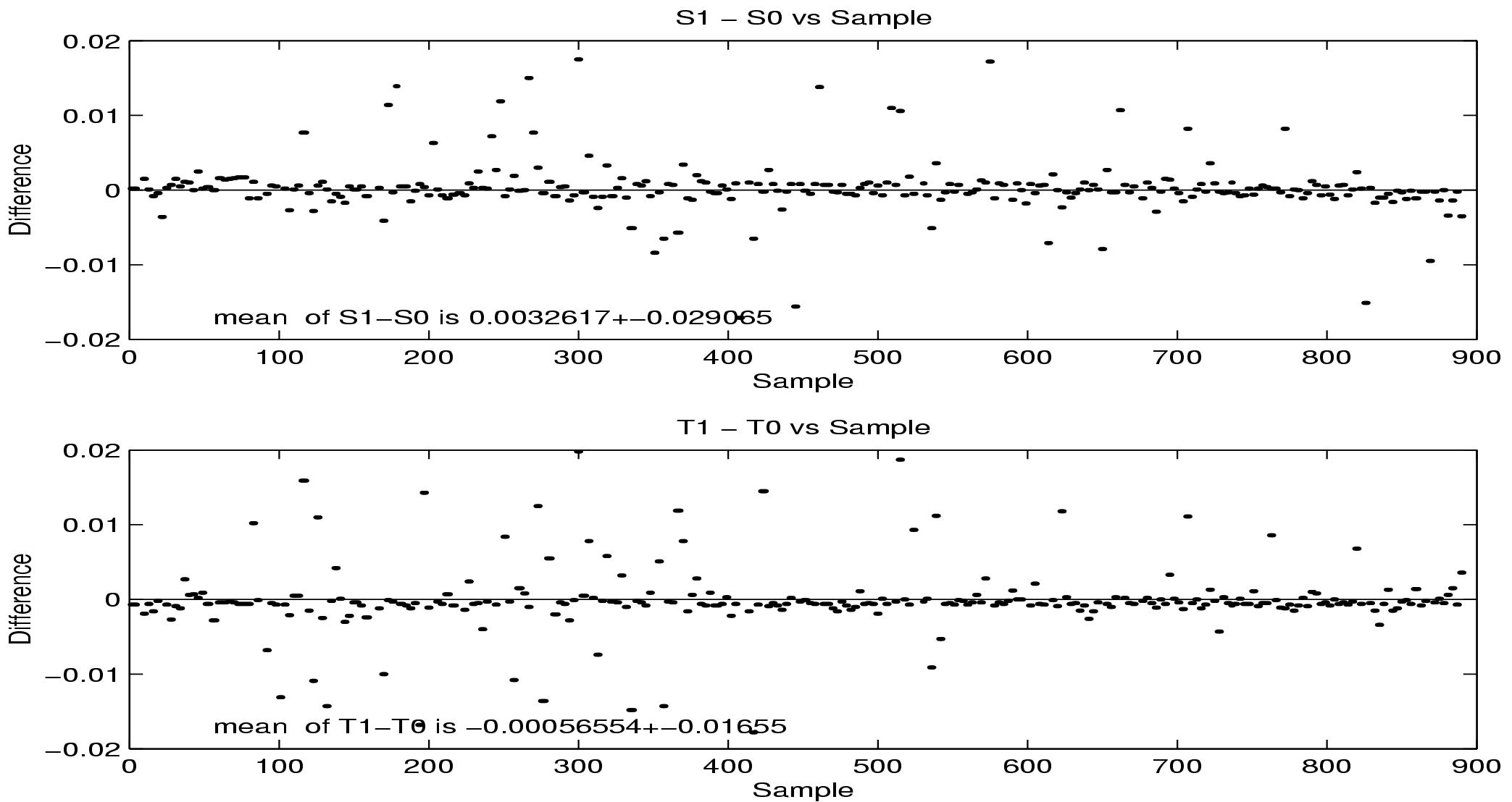
Figure3. Comparison of duplicate conductivity and temperature sensors on the CTD. (a) Conductivity
sensor difference, in terms of the calculated salinity. (b) Temperature sensor difference in degree C.
The primary instrument used for hydrographic measurements was a SeaBird 911+ Niskin/Rosette conductivity-temperature-depth (CTD) sensor system. The CTD included dual sensors for temperature and conductivity. Other sensors mounted on the CTD Rosette measured dissolved oxygen concentration, optical transmission (water clarity), fluorescence, and photosynthetically active radiation (PAR). Most CTD casts descended to within 5 m of the bottom. At stations less than 500 m deep, a Fast Repetition Rate Fluorometer (FRRF) was mounted on the Rosette. At many deeper stations, a second cast was made to 100 m to get a FRRF profile (no bottles were closed on these casts). At most stations, a new CTD-mountable Microstructure Profiling system (CMiPS) was also mounted on the Rosette. In all, 107 CTD casts were made (see Appendix 2 for details).
The 24-place Rosette was equipped with 10-liter Niskin bottles. For most casts, 23 bottles were used (the FRRF replaced the bottle in slot 23). The number of discrete water samples varied with different stations (for details see Appendix 3). Water samples were taken at the surface, 5, 10, 15, 20, 30, 50, 75 and 100 m. Other samples were taken at the oxygen minimum, the bottom, and at other interesting features below the pycnocline. The remaining bottles were distributed uniformly to get good coverage of sub-pycnocline nutrients.
Water samples were taken from these bottles for several purposes. Some samples were used to measure salinity and oxygen as a check on the CTD sensors. A water sample was taken from each bottle to measure nutrients (as described below). Samples from near-surface bottles were taken to measure chlorophyll and primary production. On a few occasions, large volumes were taken from near surface samples for genetic studies.
The two conductivity sensors on the CTD were used to calculate independently salinity, labeled S0 and S1. These values, at times when the bottles are closed, were compared to reveal any differential drift in the conductivity cells over the period of the cruise (Figure 3a). The sensors were in good agreement over the entire cruise period; the mean different was 0.0033 and the standard deviation was 0.029.
The two temperature sensors on the CTD, labeled T0 and T1, were also compared. No differential drift was evident over the period of the cruise (Figure 3b). The mean difference was -0.00056 and the standard deviation was 0.016.
The accuracy of the conductivity sensors was determined from water samples taken from three Niskin bottles from each CTD cast on which bottles were tripped, amounting to about 320 samples. These samples were typically from the surface, the halocline, and the deepest depth reached by the CTD. Samples were allowed to reach room temperature, typically taking 12 to 24 hours; the salinity was determined by a laboratory salinometer.
Two Guildline Autosal (Model 8400B) laboratory salinometers on the RVIB N. B. Palmer were used to measure the conductivity ratio, standardized against Standard Seawater. A logging computer recorded these ratios and calculated salinity.
The salinity from the Autosal was compared to the salinity calculated from each conductivity cell on the CTD. These values were automatically recorded when the bottles were closed (found in the processed .btl files and detailed here in Appendix 4). The difference is plotted against Autosal sample numbers (which were assigned consecutively during the cruise and are proxies for time) to show any drift in the accuracy of the conductivity cells (Figure 4a). Accuracy was also plotted against depth (figure not shown) and against salinity (Figure 4b).
The mean difference between salinity S0 and the bottle salinity (Sb) was -0.0000115 with a standard deviation of 0.006. The mean difference between salinity S1 and Sb was -0.0000172 with a standard deviation of 0.006. These differences are very small in comparison with the accuracy of the CTD sensor (about 0.003). There was a trend for positive differences (higher CTD sensor values) towards the end of the cruise. This difference is very small and is likely due to one Autosal session during which there was a problem establishing a correct calibration of the Autosal with Standard Seawater.
The difference between each CTD sensor and bottle salinity as a function of CTD salinity (Figure 4b) showed a trend. The largest differences were found at intermediate salinities (between 33.9 and 34.6). These salinities were mostly found in the samples taken from the halocline, where salinity was changing rapidly. The distance between the bottle and the conductivity sensor (about 0.5 m) may account for some of the discrepancy. There may also have been incomplete flushing of the bottles in these high gradient regions. The differences are small in any case.
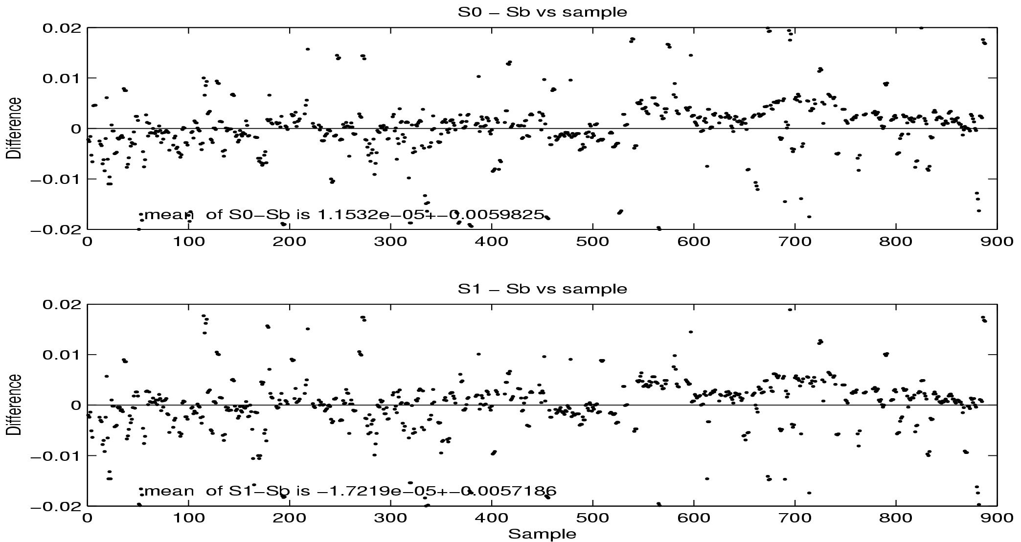
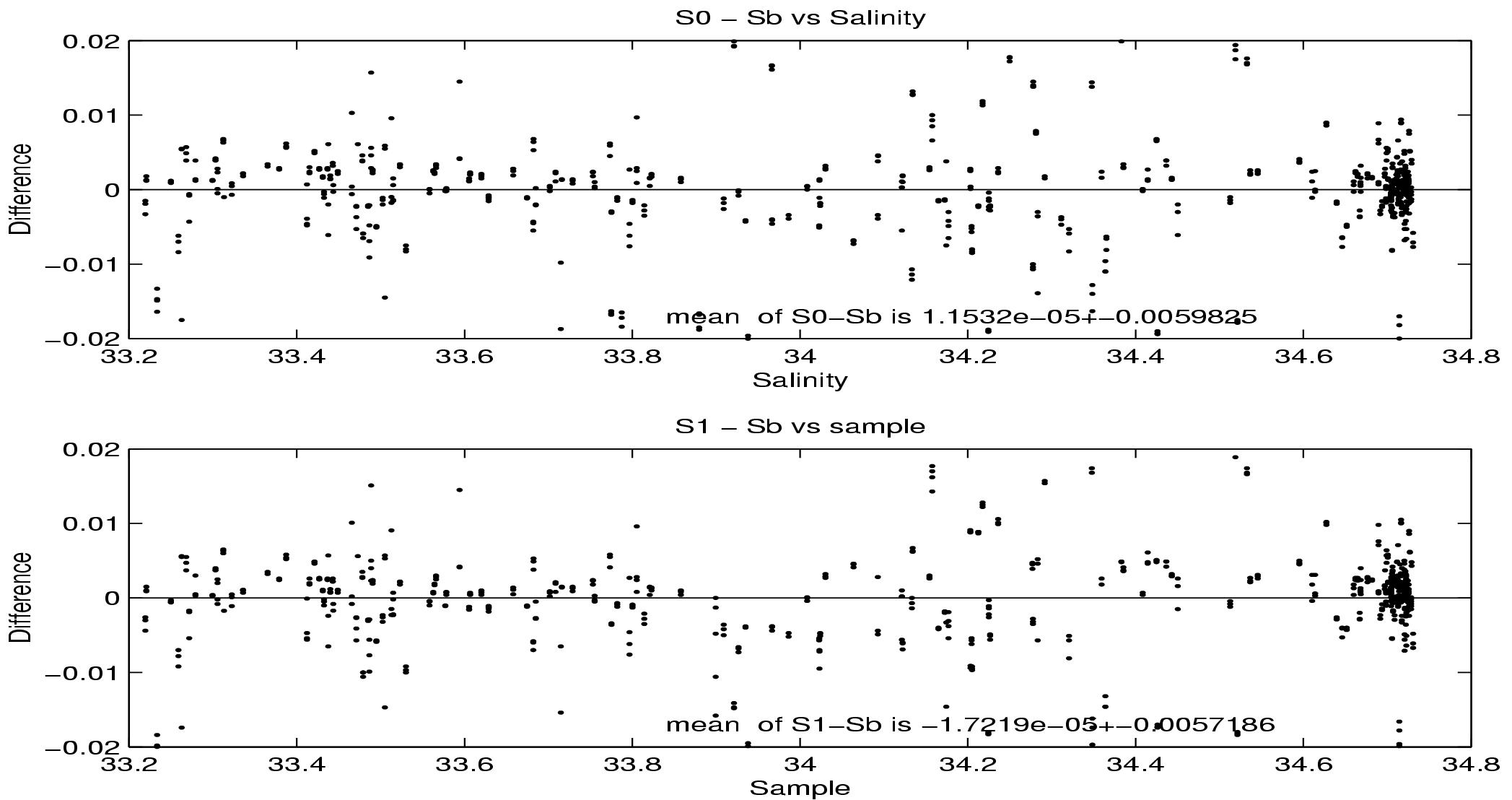
Figure 4. Comparison of the two conductivity sensors, in terms of
the calculated salinity, to the Autosal measurements of water
samples. (a) Conductivity sensor salinity minus bottle salinity
versus sample number. (b) Conductivity sensor salinity minus
bottle salinity versus salinity.
Water samples were taken for comparison with the dissolved oxygen sensor on the CTD. A total of 107 CTD casts were made that resulted in 353 water samples taken from 96 casts (Appendix 5). Water samples were not taken on short FRRF casts when the Niskin bottles were not closed.
Samples were analyzed on board usually within 48 hours of collection, using an automated amperometric oxygen titrator developed at Lamont-Doherty Earth Observatory. Four readings were lost when the titrator failed to reach an equilibrium.
After Cast 40 on 23 April, bubbles began to form in the samples taken. Tests were performed to see if the bubbles were due to air introduced during processing of samples. This possibility was eliminated, as well as other potential errors in sample collection, leaving the alternative that the gas in the bubbles was coming out of solution. We concluded that the problem probably lay with the fixing reagents; however, increasing the amount of fixing agents used did not improve matters. Of the 349 water samples, 136 had bubbles and 213 had no bubbles.
For the samples with no bubbles, comparison of the titrated oxygen values with the corresponding values from the oxygen sensor on the CTD showed a tight linear relationship (r2 = 0.987, see Figure 5). Examining the residuals, there were two outliers, and data for the practice cast (Cast 1) showed marginally higher values than for subsequent casts. Without these data, a better fit was obtained (r2 = 0.995). The estimated linear relationship was:
O2(titrated) = 1.121 O2(sensor) - 0.2625
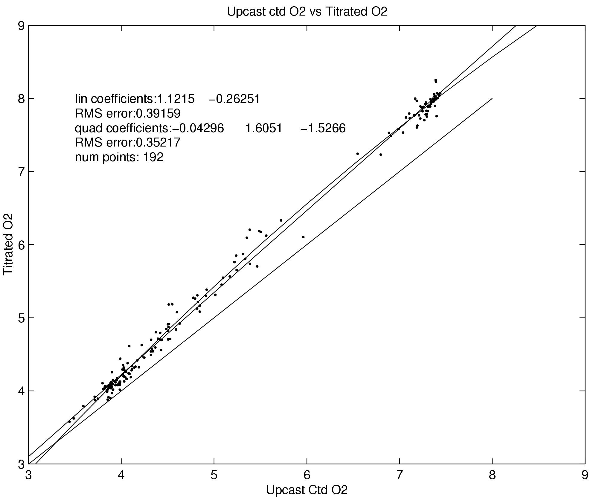
Figure 5. Oxygen sensor comparison to titrated oxygen. The green line is the
one-to-one curve. The blue line is a linear fit to the titrated values as a function of the
value reported by the CTD oxygen sensor reported at the time of bottle closing. The
dark line is the quadratic fit.
The estimate for the intercept departed significantly from 0 (t-test, alpha = 0.05, df = 190), and the slope of the relationship also departed significantly from the expected value of 1, indicating that the titration and/or sensor data were biased.
Examining the possibility of bias in the titration data due to bubble formation, we found that data taken from a subset of the samples with bubbles departed little from the relationship estimated using samples with no bubbles. Furthermore, the range of values for the titration data corresponded to that found during the earlier GLOBEC 2001 cruises. With no evidence of bias in the titration data due to the effect of bubbles, we concluded that the deviation from the expected value of 1 in the relationship between oxygen values taken by titration and by sensor was due to the sensor. The deviation can be corrected using the linear relationship estimated.
Expendable Bathythermographs (XBT) and expendable CTDs (XCTD) were used to increase the number of profiles between stations, to make rapid measurements at closely spaced stations and to measure the water structure in Drake Passage. The bulk of the XBTs were used in Drake Passage, specifically 39 probes were used at 36 stations on the southbound trip and 22 XBT probles and 3 XCDTs were used at 20 stations on the northbound trip. An additional 30 XBTs and 3 XCTDs were used in the sampling grid. Details of each of these uses is in Appendix 6.
Thirty XBT probes were used between the following station pairs (9-10, 20-21 and 50-51) to provide additional information about temperature structure near stations where warm UCDW was detected.
Two XCTDs were used at stations 67 and 69 to fill information in a high density transect across the southern side of the ACC.
A certain number of expendable probes failed due to a variety of reasons. On this cruise, we used 89 probes to get 70 profiles yielding a failure rate of 17%.
No intercomparisons were made between CTD, XCTD and XBT instruments. The first SO GLOBEC cruise (NBP01-03) made simultaneous measurements with these instruments and found no differences among them.
The microstructure profiler CMiPS (CTD-mountable Microstructure Profiling System) was used to obtain measurements of small-scale structure in the ocean due to processes such as shear instabilities, tidal stirring, mesoscale eddies, and double diffusion. Vertical diffusion through the permanent pycnocline has been suggested as an important process for heat, salt, and nutrient transport upward into the surface layer.
The CMiPS package carries two FP07 thermistors, a SeaBird SE07 microconductivity probe and a Keller pressure transducer with analog electronics to produce the following signals: (1) temperature from the first thermistor,T1, (2) temperature plus its derivative, T1+dT1/dt, also from the first thermistor, (3) similarly, T2+dT2/dt, from the second thermistor, (4) pressure, P, from the pressure transducer, (5) pressure plus its scaled derivative defined as P+57*dP/dt, and (6) conductivity and its scaled derivative, C+1.59*dC/dt, from the SE07 sensor. These signals are low pass filtered and presented to a 16-bit analog-to-digital converter where they are each sampled at a rate of 512 per second.
The instrument, which was new for this cruise, is housed in two metal cylinders which were mounted inside the Rosette on the CTD with the temperature and microconductivity probes positioned 7.5 cm up from the bottom of the CTD frame. The original plan was to mount CMiPS on the outside of the frame but it was felt that the advantages of protection for the sensors and ease of passing through Baltic Room door outweighed any disadvantages caused by the possible wake from the CTD frame. Initially, there also were concerns about risk to the sensors during installation and removal of CMiPS from the CTD frame; this turned out not to be a problem.
There was one initial problem with CMiPS due to a fault in the solid state disc drive used to store the data. This problem required the use of a conventional hard disc for the first 9 profiles of the cruise. The disadvantages of this drive were higher power consumption and introduction of a burst of noise in some of the data channels every 10 seconds when data was written to disc. After station 13, the solid state disc was able to be used by installing a floppy disc drive to boot the system which was then able to log data to the solid state drive. This worked reliably for the remainder of the cruise and power consumption was sufficiently low that only one set of batteries was required.
Data were acquired at 81 of the 92 stations on the grid and at stations MBCTD and the Marguerite Trough series of 5 stations as well as the final station in Crystal Sound. CMiPS was removed from the CTD at various times during the cruise when the water depth exceeded its 2000 m limit. At these times, temperature sensors were replaced and the conductivity sensor was examined with a microscope for signs of fouling. There were some problems with the longevity of some of the temperature sensors, so during the cruise data were collected with all of the 5 available sensors installed 2 at a time to allow cross calibration with the CTD.
In total 1.6 gigabytes of data were obtained. This includes the time for the upcast and deployment and recovery as the instrument logs at all times when it is turned on. At regular intervals the data were downloaded to a laptop computer using a 10 base T ethernet port in the instrument and data were subsequently uploaded to the ship's network for storage. CMiPS provides an analog temperature signal to one of the analog inputs on the SeaBird CTD which was logged by the CTD. This allows time alignment of the two sets of data for later analysis.
The RDI 150 kHz Acoustic Doppler Current Profiler (ADCP) system mounted in the hull of the RVIB N.B. Palmer collected data from 0011 GMT on 11 April 2002, while we crossed the Drake Passage. The system continued to collect data until we reached the Argentine EEZ (18 May) on our way back to Punta Arenas, Chile. The system was configured to acquire velocity measurements using fifty eight-meter depth bins and five minute ensemble averages. This configuration provided velocity measurements from the first bin at 31 m to 300 to 400 m, depending on scatterer and sea state. Depth bins two through ten were used with navigation to remove the ship's motion.
The ADCP was manually set to bottom track mode whenever water depths were less than 500 m. Bottom tracking was disabled during times when the survey extended beyond the continental shelf edge and into deeper waters for several hours. The Raytheon ET's were responsible for switching the ADCP tracking mode.
Preliminary processing of the ADCP data was done during the cruise using an automated version of the common Oceanographic Data Access System (CODAS) developed by E. Firing and J. Hummon from the University of Hawaii. Maps of the ADCP-derived current vectors along the ship track were generated at daily intervals at eight different depth bins using one hour ensembles. Although the system ran continuously, there are sporadic gaps of one or two hours in the data output at the beginning of the survey, probably due to heavy seas. The largest data gap for this cruise lasted about 12 hours on 21 April 2002 due to heavy seas. In addition, there were few observations during the southernmost transect (stations 89-92) due to heavy sea ice. In most shallow areas, currents below 125 m show a suspicious tendency to be aligned with the navigation track, pointing opposite to the ship's direction of travel. This may be due to insufficient removal of the ship's movement. A few large current vectors were also removed from surface (above 125 m) measurements. A final assessment of the ADCP data will be done after the cruise.
1.2.5 Meteorology Measurements
Underway meteorological observations were collected to document surface conditions during the cruise and to characterize surface forcing in the study area. All sensors were active once we left the Argentine EEZ (April 11) until we returned north to the same EEZ (May 18).
The following instruments collect observations and store them on the ship's data acquisition system. All data were stored at one minute intervals. A pair of Belfort propeller/vane anemometers were mounted on the science mast, one on each side of the ship. Three optical sensors were mounted on the mast to measure shortwave, long wave, and photosynthetically active radiation (PAR). Sensors to measure air temperature, relative humidity and pressure were mounted at the base of the mast.
Surface water conditions were measured from a water inlet in the stern thruster housing. A thermosalinograph and fluorometer provided salinity and chlorophyll, respectively. A thermometer was placed near the intake to provide sea surface temperature.
Four general results are presented here: water masses, spatial patterns, microstructure and surface fluxes. These results were obtained from analyses of the observations as they were taken, in part to make sure that the measurements were meaningful. Some of these results are consistent with measurements taken on earlier cruises and thus are confirmations of earlier ideas about processes.
1.3.1 Water Mass Distributions
The water masses in the region are clearly indicated on a potential temperature - salinity (θ - S) diagram (Figure 6) constructed from all CTD observations. Much of the surface water (lower left of figure 6) is close to the surface freezing point. Antarctic Surface Water (AASW) is water above the permanent pycnocline (generally above 100 m) and is strongly changed over the seasons by surface warming or cooling and ice freezing or melting. Many stations had a Winter Water layer, which is indicated by a subsurface temperature minimum (colder than -0.5 and salinity between 34.0 and 34.2). Oceanic Upper Circumpolar Deep Water (UCDW) appeared as a temperature maximum (about 2.0 C and salinity of 34.6). A similar Tmax was observed on the shelf at a lower temperature (1.0 to 1.5 C) at about the same salinity. This water was designated Modified CDW. Offshore of the shelf break at depths of 800 to 1000 m was Lower Circumpolar Deep Water (LCDW), which is distinguished by the salinity maximum at temperatures around 1.5 C and salinity 34.7.
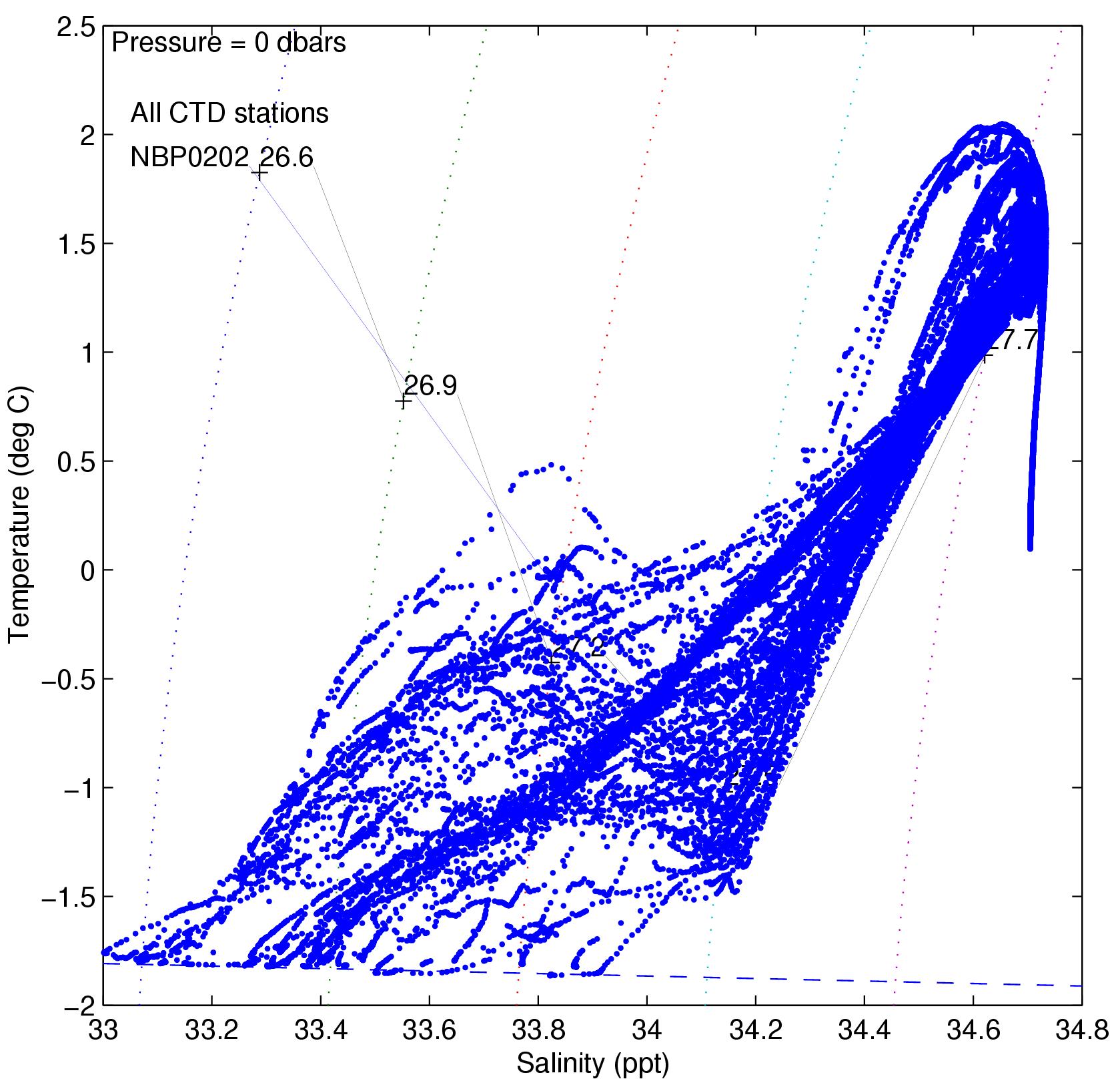
Figure 6. Potential temperature - Salinity plot for cruise data. The one meter resolution data
from the CTD casts at the 90 stations on the survey grid are used to produce this figure.
Potential temperature is calculated relative to 0 db. The dashed blue line is the freezing point.
The dotted lines are isopycnals at 0.3 kg/m3 intervals.
The appearance of surface waters near the freezing point means that the fall season was far along and conditions were approaching those of winter. The ultimate winter condition of surface water is to be at the freezing point with salinity between 33.8 and 34.0. Many stations had relatively warm water below 30 m depth and relatively low salinity. Thus, considerable heat remained in the surface ocean which will be lost to the atmosphere in the coming month. The surface salinity will be increased by haline expulsion from freezing seawater.
1.3.2 Spatial Distributions and Circulation
The spatial distribution of water properties is used to estimate water circulation and the location of exchanges between the offshore ACC and the shelf waters. The indirect estimates of circulation are augmented by ADCP measurements from the ship.
One purpose of the large-scale survey is to determine the physical structure of the shelf ecosystem. Two descriptions of this distribution are presented here: the temperature at the subsurface Tmax and the dynamic topography.
Water temperature is a good tracer of oceanic water, since it is somewhat warmer than the shelf water; the dividing isotherm is roughly 1.5 C. The temperature of the Tmax below 200 m (to avoid solar warmed water in the surface layer) showed the oceanic water (1.8 to 2.0 C) all along the shelf break (Figure 7). A plume of warmer water intruded onto the shelf west of Adelaide Island (between 400 and 450 km alongshore distance). A plume of warm water has been seen in this location at the previous two GLOBEC cruises and may be tied to the Marguerite Trough, or perhaps enters northeast of this trough. A second area of warmer water was seen in the center of the study region, but it is unclear if this water was intruding from the ocean, or intruded further to the northeast and had drifted around the gyre (described below). There was little subsurface warm water, and thus little oceanic influence, within Marguerite Bay or on the inner shelf on the southern half of the grid.
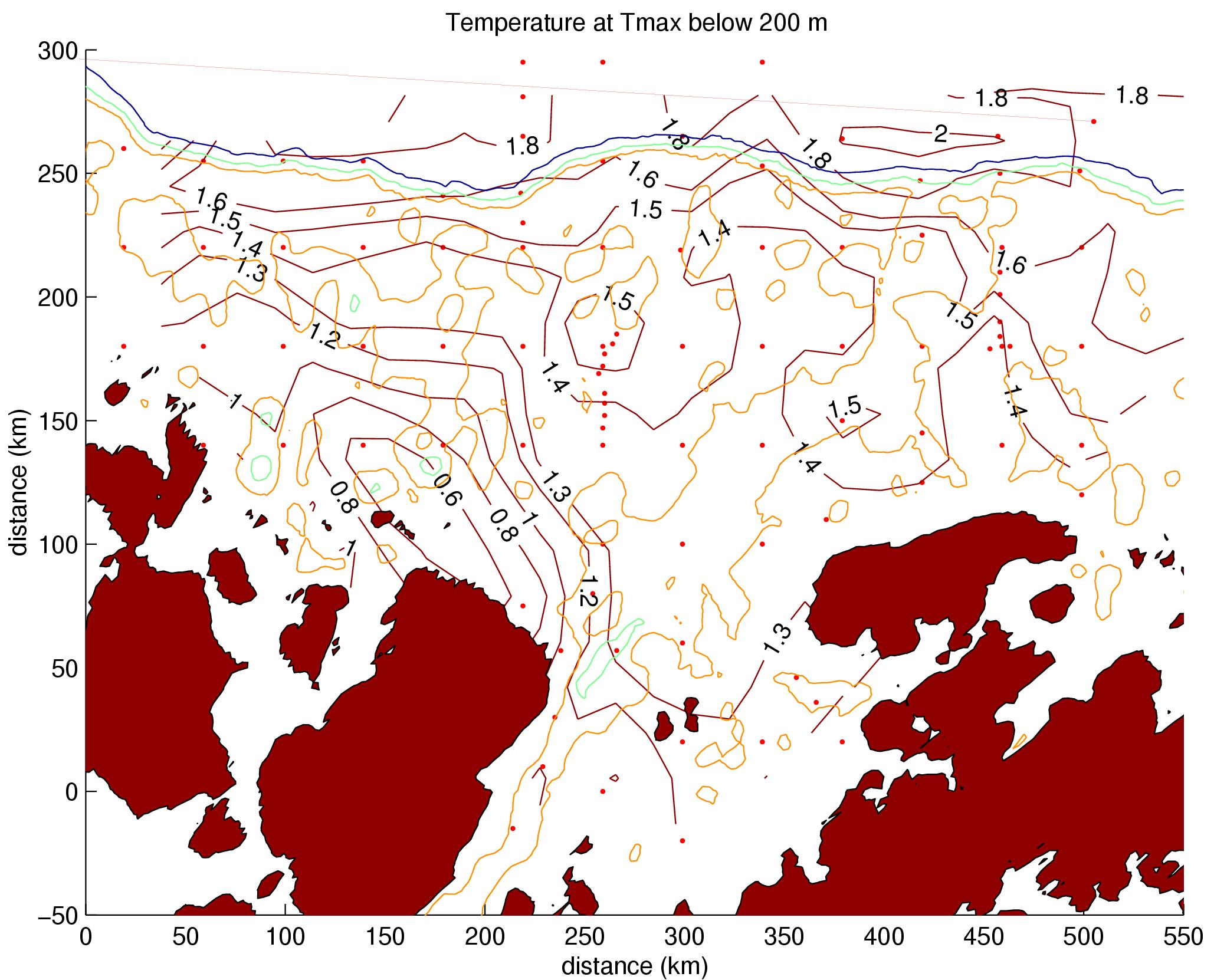
Figure 7. Potential temperature at temperature maximum below 200 m constructed from
CTD, XCTD and XBT measurements. Dark, labeled, lines are temperature contours with an
interval of 0.1 C. Dots indicate sample locations. The lighter lines are isobaths (500, 1000,
1500 m). Dark shading shows land.
The dynamic topography, the vertical integral of the density anomaly, is a more traditional indicator of circulation which uses the geostrophic balance (horizontal pressure gradients balance the Coriolis acceleration). For this shelf, the vertical density variation is weak and the shelf is relatively shallow (generally less than 500 m), which produces a weak dynamic topography. However, a clear pattern appeared in the dynamic topography calculated at the surface relative to 300 m (Figure 8). A similar pattern was seen in the 0/400 m topography (figure not shown). The sense of the circulation was clockwise around low values of dynamic topography. Flow was southwestward along the inner shelf with a strong onshore flow west of Adelaide Island and a compensating offshore flow west of Alexander Island (between 150 and 250 km alongshore distance). There was indication of two anti-clockwise circulations in Marguerite Bay, although it might be an hourglass shaped single gyre. The ACC normally flows northeastward along the shelf break, although from this cruise, the ACC seems to have a convoluted shape so flow at some places on the shelf break was backwards (southwestward).
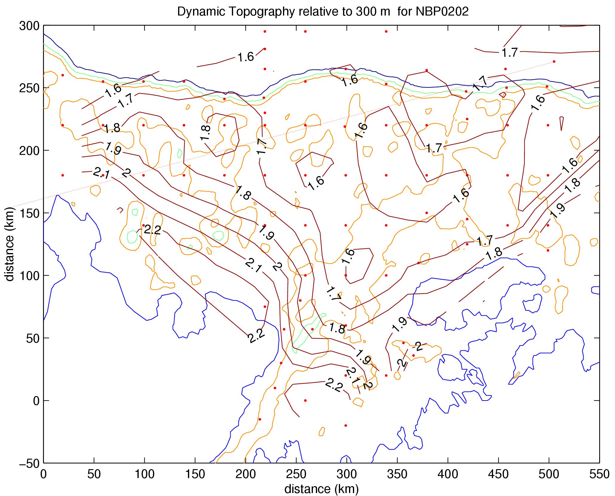
Figure 8. Dynamic topography at the surface relative to 300 m constructed from CTD and XCTD
observations. The dark numbered lines are isopleths of dynamic topography (dynamic meters) with
a contour interval of 0.1 m. Dots indicate sample locations. The lighter lines are isobaths (500, 1000,
1500 m). The heavy lines show the coastline.
An estimate of the speed of this flow was obtained from the horizontal difference of dynamic topography (the units are meters) divided by the horizontal distance and the Coriolis parameter (about .0001 s-1). A fast flow was seen coming out of the southern half of Marguerite Bay; the speed was 8 cm/s (7 km/day). A faster flow entered the shelf on the north end of the study area at 12 cm/s (10 km/day).
The ADCP records confirmed this general pattern of flow, although the data had much more spatial and temporal variability (Figure 9). The general pattern was northeastward flow along the shelf break and southwestward along the coast and into Marguerite Bay. There were some indications of variations of this flow pattern at some places, but this may have been due to temporal variations due to wind forcing changes or tides. The median flow speed from the ADCP was 6 cm/s in the upper layers and 5 cm/s at middepths. The ACC flow was observed by ADCP to be about 15 cm/s. There was a strong coastal flow south of Adelaide Island and into Marguerite Bay with speeds of 40 to 50 cm/s.
Figure 9. One hour averaged vectors in two depth ranges are shown for the duration of
the cruise.
The microstructure sensor, CMiPS, produces a large volume of data for each cast. Since this instrument is new, analysis software has yet to be developed. A quick analysis of data indicated that sensors were observing small scale variations.
A few samples of the observations were returned to Dr. Rolf Lueck, the instrument designer, for analysis. It was determined that the sensors were working as expected. A few events in these records were identified as possible microstructure due to double diffusive layering. This analysis requires calibrating the CMiPS records with the CTD record in order to estimate the density ratio and other parameters. Analysis of the full data record will proceed once the data are returned to Drs. Rolf Lueck and Laurie Padman. One problem, a low frequency (15 Hz) signal, was detected, which was thought to be due to a wake from part of the ctd frame. Modifications were made to the frame to see if this was the cause; results depend on analysis to be done after the cruise.
Description of Cruise Weather and Surface Forcing
Surface meteorological conditions were collected during the cruise at 5 min intervals over the whole region of the large scale survey during 13 April-10 May (YD 103-130) (Figure 10). This information was sufficient to estimate surface wind stress and heat flux (Figure 11). Weather conditions varied during the cruise. A flavor of this variation is provided by the descriptions below of two time periods which were characterized by weak and strong surface cooling, respectively.
Figure 10. Meteorological conditions over the cruise using 5 minute averaged observations. (a) Wind speed (m/s).
(b) Wind direction (pointing into the wind in degrees true. (c) Air
(blue) and water (red) temperature (degree C). (d) Relative humidity (percent).
(e) Surface pressure (millibars). (f) Short wave (blue) and long wave (red) radiation
(W/m2).

Figure 11. Surface fluxes over the cruise. (a) Surface stress (N/m2)
pointing in the direction the wind blows. (b) Magnitude of the wind
stress (N/m2). (c) Wind stress direction (degrees true). (d) Net surface
heat flux (W/m2) is the sum of latent, sensible, short and long wave
fluxes. Positive flux will heat the ocean. (e) Short (blue) and long
(red) wave fluxes (W/m2). (f) Sensible (blue) and latent (red) fluxes
(W/m2).
For a large part of the survey, the net surface heat flux was near zero. This period extended from the beginning of the survey (station 1, 13 April - day 103) to the southern end of Marguerite Bay (station 71 2 May - day 122). A low pressure system covered the area during these times and the skies were mainly overcast. During this period, the mean wind speed was 8 m/s and air-sea temperature difference was very small (-0.10 C) resulting in a small sensible heat flux of 2 W/m2 (Table 1). The latent heat flux, Q_lat was also small due to the low average air temperature (-0.87 C) and a high relative humidity (94%). The shortwave radiation decreased continuously as the austral winter approached. Even then, the net shortwave radiation on some days was comparable to the net long wave radiation during the daylight hours; there were even small periods when the net heat flux was zero or positive (maximum of 88 W/m2). For the weak cooling period, 96% of the net heat flux loss was due to net long wave flux.
Table 1. Surface heat budget summary for the time period 13 April to 2 May. Units are
watts/m2.
Flux Mean STD MIN MAX
Net -41 41 -203 88
Short wave 8 17 0 138
Long Wave -49 28 -156 -6
Sensible 2 10 -42 42
Latent -2 10 -47 24
A stronger heat loss was observed in the area south of Marguerite Bay. Clear sky conditions predominated for this period with high barometric pressure (maximum of 1012 mb). For this reason, net long wave was the dominant process in the surface heat flux (Table 2). Sea ice was present during most of the time; sea surface temperature was near freezing (mean of -1.67 C). Air temperature decreased significantly (mean of -7.47 C) leading to a relatively large air-sea temperature difference (-5.80 C) and a mean sensible heat flux of -79 W/m2. The mean long wave heat flux was high (-108 W/m2) due to the clear skies. The mean shortwave heat flux was small (2 W/m2) and was not a significant contributor to the net heat balance. The mean latent heat flux was -47 W/m2, mostly due to the low sea temperature and high relative humidity (86%). The average net heat flux for this period was a loss of 232 W/m2. To put these rates in perspective, surface cooling at 200 W/m2 for 5 days will cool a 25-m deep mixed layer by 0.84 C.
Table 2. Surface heat budget summary for the time period 13 April to 2 May. Units are
watts/m2.
Flux Mean STD MIN MAX
Net -232 115 -482 29
Short Wave 2 6 0 47
Long Wave -108 46 -172 -28
Sensible -79 51 -207 1
Latent -47 23 -110 0
Much of the credit for the high quality hydrographic observations collected during NBP02-02 goes to the Raytheon marine technicians: Jennifer White, Steve Tarrant, and Stian Alesandrini; and electronic technicians: Romeo LaRiviere and Sheldon Blackman. Their willing and cheerful response to all requests made collection of these data a pleasure. We also recognize efforts by deck hands Sam Villanueva, Bienvenido (Ben) Aaron and Ric Tamayo, who endured cold tedium to obtain these data. To all of these individuals, we extend our appreciation.
UNESCO, 1991. Processing of Oceanographic Station Data. United Nations Educational, Scientific and Cultural Organization, Paris. 138 pp.
2.0 Nutrients (Kent A. Fanning [PI not present on cruise], Robert T. Masserini Jr., Yulia Serebrennikova)
In addition to temperature and salinity, dissolved inorganic nutrients (nitrate, nitrite, phosphate, ammonia, and silica) are important tracers of the circulation of waters in and around Marguerite Bay. Deeper water upwelling to shallower regions close to the peninsula should be traceable by higher nutrient signatures. Nutrient concentrations nearer to the sea surface are important to physical/chemical modeling of the fate of plankton in the region that sustain krill, both as "targets" to be explained by nowcasting and as starting points for forecasting.
Analytical methods used for silica, phosphate, nitrite, and nitrate follow the recommendations of Gordon et al. (1993) for the WOCE WHP project. The analytical system we employ is a five-channel Technicon Autoanalyzer II upgraded with new heating baths, proportional pumps, colorimeters, improved optics, and an analog-to-digital conversion system (New Analyzer Program v. 2.40 by Labtronics, Inc.) This Technicon is designed for shipboard as well as laboratory use. Silicic acid is determined by forming the heteropoly acid of dissolved orthosilicic acid and ammonium molybdate, reducing it with stannous chloride, and then measuring its optical transmittance. Phosphate is determined by creating the phosphomolybdate heteropoly acid in much the same way as with the silica method. However, its reducing agent is dihydrazine sulfate, after which its transmittance is also measured. A heating bath is required to maximize the color yield. Nitrite is determined essentially by the Bendschneider and Robinson (1952) technique in which nitrite is reacted with sulfanilamide (SAN) to form a diazotized derivative that is then reacted with a substituted ethylenediamine compound (NED) to form a rose pink azo dye which is measured colorimetrically. Nitrate is determined by difference after a separate aliquot of a sample is passed through a Cd reduction column to covert its nitrate to nitrite, followed by the measurement of the "augmented" nitrite concentration using the same method as in the nitrite analysis.
In the analytical ammonia method, ammonium reacts with alkaline phenol and hypochlorite to form indophenolblue. Sodium nitroferricyanide intensifies the blue color formed, which is then measured in a colorimeter of the nutrient-analyzer. Precipitation of calcium and magnesium hydroxides is eliminated by the addition of sodium citrate complexing reagent. A heating bath is required. Our version of this technique is based on modifications of published methods such as the article by F. Koroleff in Grasshoff (1976). These modifications were made at Alpkem (now Astoria-Pacific International, Inc.) and at L.Gordon's nutrient laboratory at Oregon State University.
Nitrate, nitrite, phosphate, ammonia, and silicic acid were measured from every Niskin bottle tripped from all hydrocasts (2035 seawater samples) on this cruise. These data are available on the cruise CDROM and will be posted to the U.S. GLOBEC Data website.
2.4 Preliminary Results for Nutrient Concentrations
Nitrate and phosphate exhibited the expected vertical distributions: high concentrations at depth overlain by slight increases just below the mixed layer followed by substantial decreases within the euphotic zone. Approximate concentrations for nitrate and phosphate (respectively) in these regions were: 33.0 and 2.32 μM (deep water), 35.3 and 2.47 μM (just below the mixed layer), and 22.5 and 1.6 μM (euphotic zone).
Nitrite and ammonia concentrations were essentially zero, here defined as less than the detection limit of the chemistries employed, below the mixed layer. Within the mixed layer the average nitrite and ammonia concentrations were approximately 0.23 and 1.9 μM, respectively. A subsurface nitrite maximum near the bottom of the mixed layer was located approximately twenty-to-forty nautical miles inshore from the furthest offshore station. The nitrite concentration within the bolus increased to roughly 0.35 μM. This offshore subsurface nitrite maximum was seen on survey lines 1-7, 9, 10, 11, and 13. However, on line 12 the feature was seen much further inshore, approximately 60 nautical miles inshore from the furthest offshore station.
Silicic acid exhibited an increase in concentration shoreward within the mixed layer. In general it also exhibited a classic nutrient structure, with average concentrations that decreased from roughly 110 μM below the mixed layer to 60 μM within the euphotic zone. One feature of note in the silicic acid data was the presence of a lens of depleted silicic acid at a depth of approximately 260 meters associated with the 1.8-degree water seen at station 9 on transect 2. This water mass had a silicic acid concentration of approximately 90 μM, or 10 μM less than the water surrounding it.
There appeared to be a nutrient frontal feature within the euphotic zone aligned generally across and penetrating about halfway into Marguerite Bay. This feature was indicated by an increase in nitrate, nitrite, silicic acid, and phosphate concentrations. The front’s position agreed well with contour maps of dynamic topography generated by other groups on this cruise. Preliminary surface contours of average mixed-layer nutrient concentrations seemed to depict a gyre on the shelf with an edge that was generally aligned across the mouth and penetrated approximately halfway into Marguerite Bay.
Within portions of the mixed layer of Marguerite Bay that are away from the influence of the gyre, ammonia exhibited an enrichment at near shore stations to a depth of approximately 50 meters. Concentrations there ranged between 2.5 and 2.9 μM. The region seemed to be closely associated with slightly fresher water found near the surface in the back of the Bay. Overall, ammonia concentrations in the mixed layer on this cruise were comparable with those of the Winter SO GLOBEC II cruise for the same region last year. Thus, they were significantly lower than those of last year’s Fall SO GLOBEC cruise values (3.5 to 4 μM) for the same region.
The mixed layer of Marguerite Bay exhibited depletions in concentrations of four of the five nutrients studied (nitrate, nitrite, silicic acid, and orthophosphate). Average shelf concentrations of nitrate, nitrite, and orthophosphate within the euphotic zone were approximately 22.5, 0.2, and 1.6 μM, respectively. Surface concentrations of silicic acid displayed more horizontal variability, increasing from about 50 μM at the furthest offshore station to a maximum of slightly more than 70 μM approximately 90 nautical miles shoreward from that station and then decreasing to 60 μM inside the Bay. Nitrate, nitrite, and phosphate declined within the euphotic zone of Marguerite Bay to roughly 18, 0.15, and 1.4 μM, respectively.
Gordon, L.I., J.C. Jennings, Jr., A.A. Ross, and J.M. Krest, A Suggested Protocol For Continuous Flow Automated Analysis of Seawater Nutrients, in WOCE Operation Manual, WHP Office Report 90-1, WOCE Report 77 No. 68/91, 1-52, 1993.
Grasshoff, K. 1976. Methods of Seawater Analysis, Verlag Chemie, Weinheim, Germany, and New York, NY, 317 pp.
3.0 Primary Production Component (Maria Vernet [PI not present on cruise], Wendy Kozlowski, Kristy Aller)
The estimation of primary production has three main objectives: (1) estimation of primary productivity rates during fall and winter in the area of study as a possible source of food for krill and other zooplanktors; (2) understanding the mesoscale patterns of phytoplankton distribution with respect to physical, chemical and biological processes; and (3) obtaining insight into the over-wintering dynamics of phytoplankton, including their interaction with sea ice communities. For this purpose, primary production was measured with two methods during this cruise: estimation of daily net production with simulated in situ experiments (SIS), and profiles with a Fast Repetition Rate Fluorometer (FRRF), with the aim to increase resolution in the sampling of phytoplankton activity and the expectation of modeling primary production with this method using 14C experiments as comparison. A third approach, that of estimating potential primary production and gaining information on the dynamics of light adaptation by means of Photosynthesis vs Irradiance curves was carried out on all ice samples collected.
During this third Southern Oceans GLOBEC cruise, we also increased our emphasis on estimation of phytoplankton biomass, with measurements of chlorophyll (chla) and particulate organic carbon and nitrogen (CHN) throughout the water column. Recording of both surface and water column photosynthetically available radiation (PAR) was carried out throughout the sampling duration of the cruise.
The FRRF was deployed at all stations where the water depth was less than 500 m, and at stations 12, 22, 37, 46, 70, and 84, a separate cast was done before the main CTD cast to a depth of 100 m for collection of FRRF data at deep water stations (Figure 12). SIS experiments were done once a day, with water generally sampled from the station closest to, but preceding sunrise in order to allow for accurate simulations of daylengths (Figure 12). Chlorophylls were sampled from all stations where the rosette was deployed, plus from a bucket sample at station 44 when the weather prevented use of the CTD, and water was filtered for POC samples at every other station sampled along the grid.
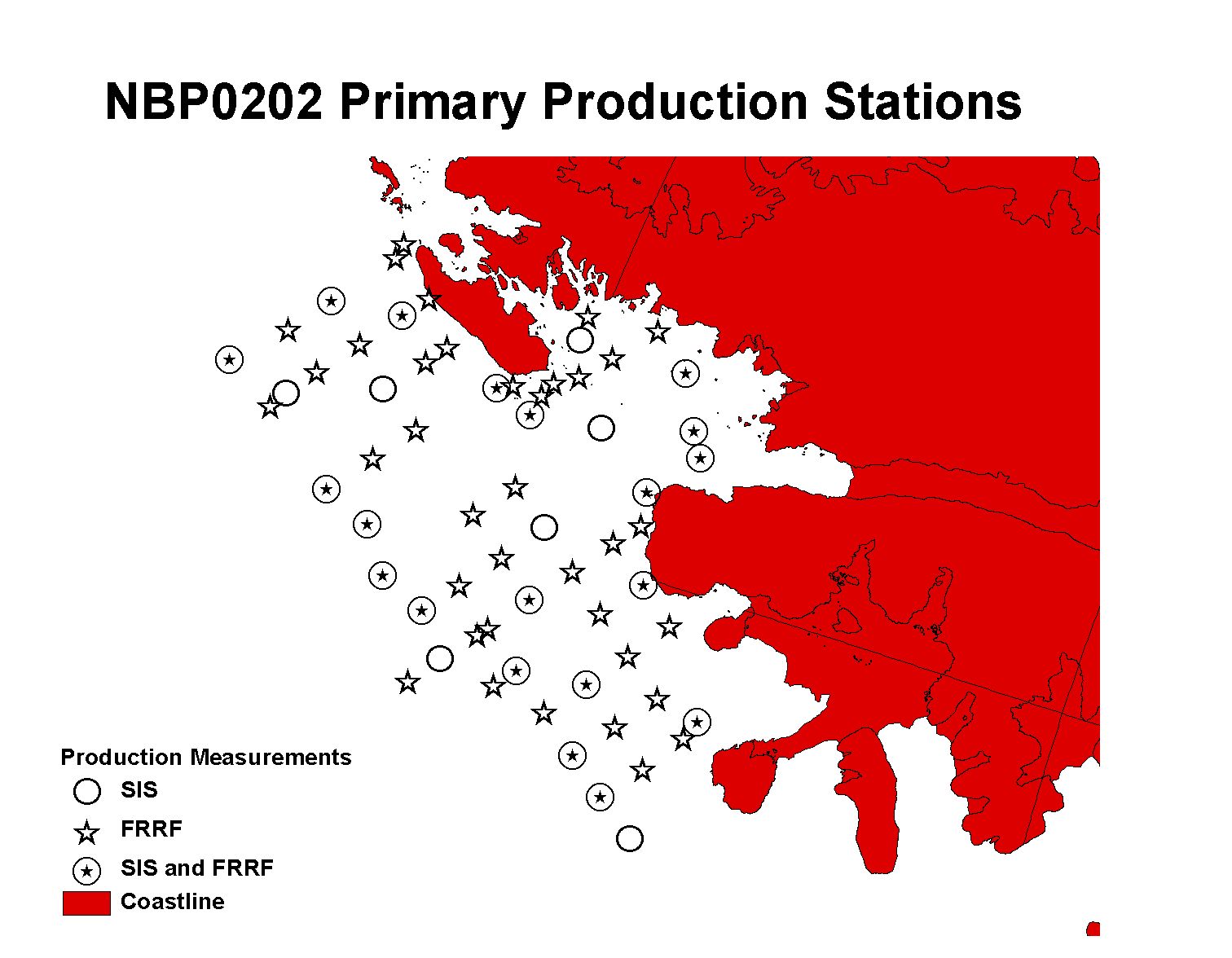
Figure 12. Map of all primary production stations sampled.
For SIS experiments water was collected from the surface, and from five, ten, fifteen, twenty, and thirty meters deep. The FRRF was deployed as part of the CTD rosette, with a descent rate of 10 meters per minute for the first fifty meters, 20 meters per minute to 100 meters in depth and 50 meters per minute for the remainder of the cast. Data was analyzed from the downcasts, to a depth of 150 meters. Chlorophylls and CHNs were collected at the same depths as for SIS experiments, plus at 50 meters, 100m, the bottom and three other intermediate depths varying based on total cast length.
Ice sampling during the cruise was generally opportunistic. See Table 3 for a summary of Ice Station Locations and Samples collected. On a few occasions, sampling was done while underway, with a bucket over the side of the ship. When the ice was larger, ice was again collected into a bucket, but using the personnel basket as a working platform. When the ice floes were large enough to core from, personnel were lowered with the basket to the ice and worked directly from the floes.
Once the ice samples were brought on board the ship, 0.2μ filtered seawater was added (to samples other than slush and pancake) to approximate a 0.33 dilution, and the ice was allowed to melt in the dark in a 2̊ C cold room. Once melted, the water was sub-sampled for chlorophylls, particulate carbon and nitrogen, and production (PI). Ice that was not diluted was allowed to melt under the same conditions, and was additionally sub-sampled for nutrients and salinity.
Chlorophylls were measured using a Turner Designs Digital 10-AU-05 Fluorometer, serial number 5333-FXXX, calibrated using a chlorophyll a standard from Sigma Chemicals, dissolved in 90% acetone. The “Fast Tracka” Fast Repetition Rate Fluorometer, serial number 182037, is made by Chelsea Instruments, and was outfitted with independent depth and PAR sensors. All data was recorded internally to the instrument, and data was downloaded directly to computer after every few casts. Incubations for the SIS experiments were done in Plexiglas tubes, shaded to simulate collection light levels with window screening, incubated in an on-deck Plexiglas tank, which was outfitted with running seawater in order to maintain in situ temperatures. PI curves were done in custom built incubators, designed to hold 7ml vials, irradiate at light levels between zero and 460 μE/m2/sec, and were attached to water baths to maintain in situ collections temperatures. CHN samples will be analyzed upon return to the States. Ice water nutrients were measured on board by USF analysts, and salinities were measured using a hand held refractometer. Light data was collected using a Biospherical Instruments GUV Radiometer, serial number 9228, mounted on the science mast, configured with a PAR channel, as well as channels for 305, 320, 340 and 380nm wavelengths. Additional PAR data was collected using a Biospherical Instruments QSR-240 sensor, serial number 6356, also mounted on the science mast.
Table 3. Summary of sea ice samples, with locations and ice types. Possible Samples collected are chlorophyll (chl), particulate carbon, hydrogen and nitrogen (CHN), Dissolved Inorganic Nutrients (DIN), salinity (salt), and Primary Production (PP).
Date |
Nearest Cons St # |
Lat |
Lon |
Sample |
Ice Type |
Samples Collected |
4/23/02 |
037 |
-68.183 |
-68.240 |
Ice1 |
pancake |
chl, CHN, DIN, 2xPP |
4/24/02 |
040 |
-68.480 |
-68.804 |
Ice2 |
slush |
chl, CHN, 2xPP |
4/29/02 |
055 |
-68.885 |
-68.976 |
Ice3A |
Core: 0-83cm |
SD, IT, chl, CHN, 1xPP |
4/29/02 |
055 |
-68.885 |
-68.976 |
Ice3B |
Core: 83-233cm |
SD, IT, chl, CHN, 1xPP |
4/30/02 |
057 |
-68.998 |
-69.429 |
Ice4A |
Core: 0-126cm |
SD, IT, chl, CHN, 1xPP |
4/30/02 |
057 |
-68.998 |
-69.429 |
Ice4B |
Core: 126-207cm |
SD, IT, chl, CHN, 1xPP |
4/30/02 |
057 |
-68.998 |
-69.429 |
Ice4C |
Core: 207-293cm |
SD, IT, chl, CHN, 1xPP |
4/30/02 |
057 |
-68.998 |
-69.429 |
Ice4S |
slush/brine |
chl, CHN, DIN, salt, 1xPP |
5/1/02 |
059 |
-68.694 |
-70.462 |
Ice5 |
slush |
chl, CHN, 2xPP |
5/5/02 |
076 |
-69.171 |
-72.754 |
Ice6A |
Core: 0-79cm |
SD, IT, chl, CHN, 1xPP |
5/5/02 |
076 |
-69.171 |
-72.754 |
Ice6B |
Core: 79-96cm |
SD, IT, chl, CHN, 2xPP |
5/5/02 |
076 |
-69.171 |
-72.754 |
Ice6C |
Core: 96-185cm |
SD, IT, chl, CHN, 1xPP |
5/5/02 |
076 |
-69.171 |
-72.754 |
Ice6S |
slush/brine |
Chl, chn, DIN, salt, 1xPP |
5/6/02 |
078 |
-68.727 |
-74.309 |
Ice7 |
slush |
chl, CHN, DIN, salt, 1xPP |
5/8/02 |
084 |
-69.233 |
-74.196 |
Ice8 |
pancake |
chl, chn, 1xPP |
5/8/02 |
085 |
-69.549 |
-74.431 |
Ice9A |
Core: 0-92cm |
SD, IT, chl, CHN, 1xPP |
5/8/02 |
085 |
-69.549 |
-74.431 |
Ice9B |
Core: 92-167cm |
SD, IT, chl, CHN, 1xPP |
5/8/02 |
085 |
-69.549 |
-74.431 |
Ice9C |
Core: 167-205cm |
SD, IT, chl, CHN, 1xPP |
5/8/02 |
085 |
-69.549 |
-74.431 |
Ice9D |
Core: 205-257cm |
SD, IT, chl, CHN, 1xPP |
5/8/02 |
085 |
-69.549 |
-74.431 |
Ice9S |
slush/brine |
chl, CHN, 1xPP |
5/10/02 |
092 |
-69.530 |
-76.323 |
Ice10A |
Core1: 0-41cm |
SD, IT, chl, CHN, 1xPP |
5/10/02 |
092 |
-69.530 |
-76.323 |
Ice10B |
Core1: 41-94cm |
SD, IT, chl, CHN, 1xPP |
5/10/02 |
092 |
-69.530 |
-76.323 |
Ice10C |
Core1: 94-146cm |
SD, IT, chl, CHN, 1xPP |
5/10/02 |
092 |
-69.530 |
-76.323 |
Ice10D |
Core2: 0-149cm |
SD, IT, chl, CHN, 1xPP |
5/10/02 |
092 |
-69.530 |
-76.323 |
Ice10S |
slush/brine |
chl, CHN, DIN, salt, 2xPP |
5/10/02 |
092 |
-69.530 |
-76.323 |
Ice10E |
Core3: 0-14cm |
DIN, salt |
5/10/02 |
092 |
-69.530 |
-76.323 |
Ice10F |
Core3: 14-41cm |
DIN, salt |
5/10/02 |
092 |
-69.530 |
-76.323 |
Ice10G |
Core3: 41-86cm |
DIN, salt |
5/10/02 |
092 |
-69.530 |
-76.323 |
Ice10H |
Core3: 86-109cm |
DIN, salt |
5/10/02 |
092 |
-69.530 |
-76.323 |
Ice10I |
Core3: 109-127cm |
DIN, salt |
5/10/02 |
092 |
-69.530 |
-76.323 |
Ice10J |
Core3: 127-146cm |
DIN, salt |
Over the course of the thirty-six science days of this trip, a total of twenty seven SIS experiments were completed. Twenty seven PI curves were run on ice from ten different locations, and the FRRF was cast (with data acquired) 57 times throughout the grid. For estimations of biomass (standing carbon stocks), both CHN and chlorophyll samples were taken. A total of 609 POC samples were collected, and 1606 chlorophyll samples were taken from the 102 sampling stations. Of those biomass samples, 30 were ice-related samples.
Surface PAR data was on all days that primary production experiments were done. GUV data was collected at one minute intervals and logged directly to computer (see Table 4 for daily measured light levels). QSR PAR data was collected as part of the JGOF meteorological data set. A comparison of the two instruments was done to continue to monitor differences between the two types (scalar vs. cosine) of sensor (see Figure 13). PAR data were also collected during each daylight CTD cast using a profiling PAR sensor, as well as on the FRRF, and will be used in conjunction with surface PAR data for the analysis of water column production.
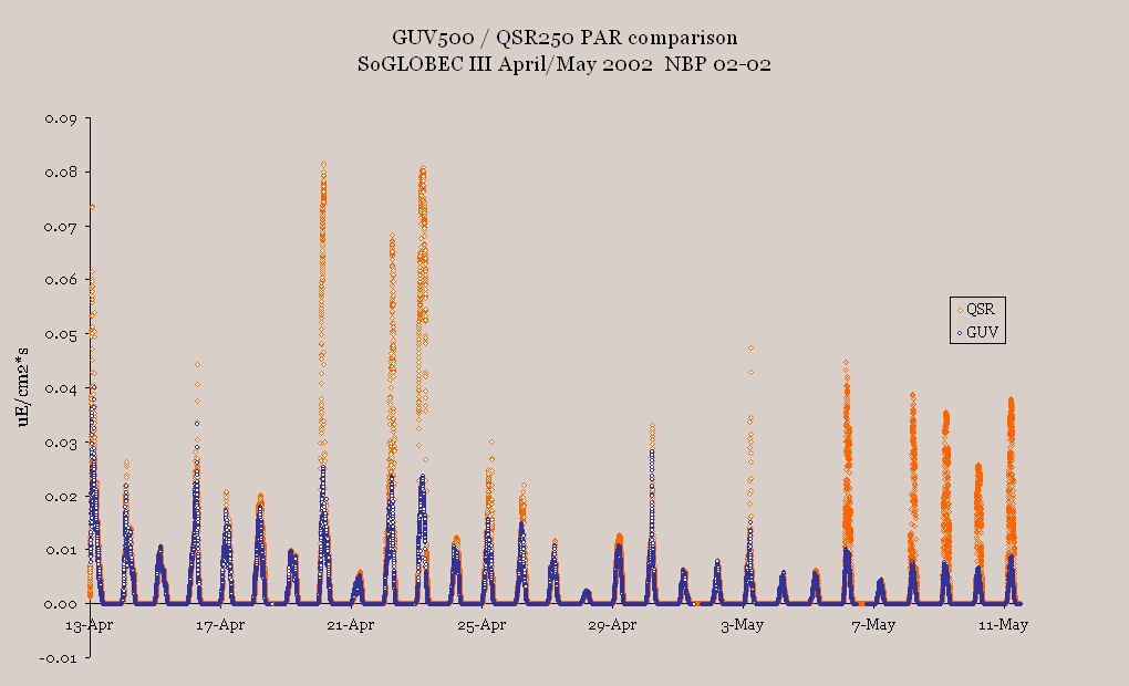
Figure 13. Plot of comparison of Biospherical Instruments QSR-240 and GUV 500 Photosynthetically
Active Radiation (400-700 nm) measurements over the course of NBP 02-02.
3.3 Preliminary Results
Final analysis is yet to be completed on the majority of the data collected on this cruise. There appears to be similar North-South and onshore-offshore trends in the chlorophyll levels as were seen in GLOBEC I and II, with slightly higher levels seen on the Northern, outside part of the grid. Higher chlorophyll levels were also seen at five stations in the North Eastern side of Marguerite Bay. Surface chlorophyll values throughout the grid ranged from 0.09 μg/l down to 2.16 μg/l, with a maximum integrated value seen at consecutive station 14 (166.28 μg/m2 integrated to 100m), and a minimum at consecutive station 56 (3.54 μg/m2). Water column primary production followed the same pattern as chlorophyll, with highest production seen on the North Western corner of the grid. Of the stations where SIS experiments were done, production estimates ranged from 8.1 mgC/m2/d at station 59, to 249.6 mgC/m2/d at station 15. All ice samples had measurable amounts of production, with several of the new pancake and brine samples showing some of the highest productions seen on the cruise.
Table 4. PAR (Photosynthetically Available Radiation, 400 – 700 nm) data, from BSI GUV500 mounted on Science Mast. Day lengths and daily irradiance values were calculated using PAR values above 0.0 μE/cm2*sec.
Date |
Sunrise |
Sunset |
Dec. Hours |
μE/cm2 |
4/14 |
11:32 |
21:45 |
10.22 |
256.70 |
4/15 |
11:35 |
21:27 |
9.87 |
160.83 |
4/16 |
11:46 |
21:37 |
9.85 |
289.22 |
4/17 |
11:47 |
21:33 |
9.77 |
223.01 |
4/18 |
11:53 |
21:30 |
9.62 |
253.48 |
4/19 |
11:55 |
21:28 |
9.55 |
154.72 |
4/20 |
11:57 |
21:33 |
9.60 |
318.51 |
4/21 |
12:18 |
21:13 |
8.92 |
74.57 |
4/22 |
11:58 |
21:18 |
9.33 |
276.75 |
4/23 |
11:54 |
21:02 |
9.13 |
363.76 |
4/24 |
12:15 |
20:50 |
8.58 |
141.10 |
4/25 |
12:24 |
21:09 |
8.75 |
197.80 |
4/26 |
12:40 |
21:22 |
8.70 |
166.96 |
4/27 |
12:41 |
20:58 |
8.28 |
126.38 |
4/28 |
12:49 |
20:25 |
7.60 |
30.82 |
4/29 |
12:27 |
20:39 |
8.20 |
160.43 |
4/30 |
12:35 |
20:37 |
8.03 |
169.28 |
5/1 |
12:54 |
20:37 |
7.72 |
66.16 |
5/2 |
13:02 |
20:47 |
7.75 |
74.31 |
5/3 |
13:00 |
20:47 |
7.78 |
107.89 |
5/4 |
13:07 |
20:34 |
7.45 |
51.41 |
5/5 |
13:12 |
20:28 |
7.27 |
63.72 |
5/6 |
13:14 |
20:44 |
7.50 |
122.57 |
5/7 |
13:41 |
20:22 |
6.68 |
43.36 |
5/8 |
13:28 |
20:26 |
6.97 |
75.95 |
5/9 |
13:34 |
20:36 |
7.03 |
92.67 |
5/10 |
13:45 |
20:22 |
6.62 |
71.51 |
5/11 |
13:26 |
20:13 |
6.78 |
92.23 |
(Peter Wiebe, Carin Ashjian, Scott Gallager [PI not present on cruise], Cabell Davis [PI not present on cruise])
The winter distribution and abundance of the Antarctic krill population throughout the Western Peninsula continental shelf study area are poorly known, yet this population is hypothesized to be an especially important overwintering site for krill in this geographical region of the Antarctic ecosystem. Thus, the principal objectives of this component of the program are to determine the broad-scale distribution of larval, juvenile, and adult krill throughout the study area, to relate and compare their distributions to the distributions of the other members of the zooplankton community, to contribute to relating their distributions to mesoscale and regional circulation and seasonal changes in ice cover, food availability, and predators, and to determine the small-scale distribution of larval krill in relation to physical structure of sea ice. To accomplish these objectives, the same three instrument platforms that were used on the first two Southern Ocean GLOBEC broad-scale cruises, were used on this cruise. A 1-m2 MOCNESS equipped with a strobe light was used to sample the zooplankton at a selected series of stations distributed throughout the survey station grid. A towed body, BIOMAPER-II was towyoed along the trackline between stations to collect acoustic data, video images, and environmental data between the surface and bottom in much of the survey area. An ROV was used to sample under the ice and to collect video images of krill living in association with the ice under surface, environmental data, and current data. This section of the cruise report will detail the various methods used with each of the instrument systems or in the case of BIOMAPER-II, its sub-systems.
4.1 Zooplankton Sampling with the 1m2 MOCNESS Net System
(C. Ashjian. P. Alatalo, G. Rosenwaks)
The 1-m2 MOCNESS net sampling of zooplankton had two main objectives. The first was to sample the vertical distribution, abundance, and population structure (size, life stage) of the plankton at selected locations across the broad-scale survey grid. The second objective was to collect information on the size distribution of the plankton, especially the krill, in order to ground-truth the acoustic and video data collected using the BIOMAPER-II multi-frequency acoustic and video plankton recorder system. Using the size distribution of planktonic taxa from different depths and locations, the acoustic intensity resulting from insonification of that water parcel will be calculated to check and ground-truth the acoustic backscatter from the BIOMAPER-II. The dominant species of the taxa enumerated using the Video Plankton Recorder also will be identified.
Sampling was conducted using a 1-m2 MOCNESS (Multiple Opening/Closing Net and Environmental Sensing System) equipped with 333 μm mesh nets and a suite of environmental sensors including temperature, conductivity, fluorescence, and light transmission probes. The fluorometer and transmissometer were removed part way through the cruise in order to transfer the options case from the MOCNESS to the BIOMAPER-II on which the options case had failed. The MOCNESS also was equipped with a strong strobe light, which flashed at 4-second intervals. Because krill are strong swimmers and likely can see slow moving nets such as the MOCNESS, krill frequently avoid capture by net systems. The rationale behind the strobe system was to shock or blind the krill temporarily so that the net would not be perceived and avoided.
Tows were conducted at 24 locations (Figure 14). Oblique tows were conducted from near bottom to the surface, sampling the entire water column on the down-cast and selected depths on the up-cast with the remaining eight nets. Typically, the upper 100 m was sampled at 25 m intervals, with 50 m intervals in the intermediate depth ranges and greater intervals (150, 200 m) in the deepest depth ranges. Samples were preserved upon recovery in 4% formalin except for the first net (water column sample) that was preserved in ethanol to be utilized for genetic analyses.
Figure 14. Location of the 1 m2 MOCNESS tows. Standard station numbers,
where available, are shown next to the symbols. Different symbols demonstrate the
presence or absence of krill and furcilia and locations where abundances of these
taxa were notably greater.
Despite the light ice cover encountered at many locations, towing was not seriously impaired. Cautionary measures were employed in ice covered regions. The wire was watched closely with a dedicated video camera to quickly observe any ice that became caught under the cable so that the ship could be stopped quickly. Also, less wire than bottom depth was utilized so that the MOCNESS would not hit the sea floor if the ship slowed or halted because of heavy ice.
Samples will be analyzed for displacement volume biomass and taxonomic and size composition of the plankton upon return to the laboratory. The taxonomic/size composition analysis will be conducted using silhouette analysis that yields size specific abundances of the different taxa (e.g., large copepod, large krill, small krill, ctenophore). These abundances and sizes then are used to extrapolate sample biomass using empirical relationships between size and biomass for each taxon. The size/taxa information also will be used to predict the backscatter that would result from insonification of this plankton community by the BIOMAPER-II acoustic transducers.
Overall, abundances and taxonomic composition were much reduced relative to those observed during the fall cruise cruise of 2001 (NBP0103) and were similar to those observed during the winter of 2001 (NBP0104). Copepods frequently were important both numerically and in terms of biomass. Very few furcilia and adult krill were seen. Only two locations in Marguerite Bay appeared to have abundant krill and furcilia; Stations 28 and 54 both of which were located along the axis of the mouth of Marguerite Bay in cold, fresh water of the “coastal” current which flows south along Adelaide Island, loops into Marguerite Bay, and exits at the southern end flowing south and west along the shelf. Sampling volumes were comparable between all of the cruises so it is likely that these qualitative observations represent relative plankton abundances on the shelf. High abundances of krill were observed in Matha Strait at the entrance to Crystal Sound, north of Adelaide Island. These high abundances were correlated with the presence of elevated backscatter observed both on the SIMRAD echosounder during the tow and with the BIOMAPER-II acoustics during a survey conducted prior to the MOCNESS tow.
Many people assisted with the MOCNESS tows and their assistance is gratefully acknowledged. Special thanks to Peter Martin, Romeo LaRiviere, Jenny White, Stian Alesandrini, Steve Tarrant, Alice Doyle, Julian Ashford, the BIOMAPER-II group, Peter Wiebe, and the bridge crew of the NBP (Capt. Joe, Val, Rich, John, Rachelle).
The BIO-Optical Multi-frequency Acoustical and Physical Environmental Recorder or BIOMAPER II is a towed system capable of conducting quantitative surveys of the spatial distribution of coastal and oceanic plankton/nekton. The system consists of a multi-frequency sonar, a video plankton recorder system (VPR), and an environmental sensor package (CTD, fluorometer, transmissometer). Also included are an electro-optic tow cable, a winch with slip rings, and van which holds the electronic equipment for real-time data processing and analysis. The towbody is capable of operating to a depth of 300 meters at 4 to 6 knots, but because of several re-terminations following damage to the electro-optical towing wire thus reducing the wire length, the operational depth on this cruise was a little over 200 m. The system can be operated in a surface towed down-looking mode, in a vertical oscillatory "towyo" mode, or in a sub-surface up/down looking horizontal mode. All three modes were used to some extent on NBP0202. To enhance the performance and utility of BIOMAPER II in high sea states, a winch, slack tensioner, and over-boarding sheave/docking assembly were used.
As on the first two SO GLOBEC broad-scale cruises (NBP0103, NBP0104), BIOMAPER-II was deployed from the stern of the RVIB N. B. Palmer. Attached to the starboard side of the A-frame on the Palmer was a stiff arm, designed and constructed at WHOI, to lower the over-boarding sheave/docking assembly to a level that would minimize the distance that BIOMAPER-II needed to be hauled up to be docked and still clear the stern rail when the A-frame was boomed in. It was shackled at two points to pad eyes on the top of the A-frame. The over boarding sheave articulated and was equipped with a hydraulic ram, so that its position could be adjusted to keep the docking mechanism vertical during launch and recovery, and to move it inboard of the wire when towing. During the port setup in Punta Arenas before this cruise, the deck plates holding the winch and slack tensioner were repositioned in an attempt to better align the cable leaving the slack tensioner with the overboarding sheave. In addition, a newly fabricated set of rollers were mounted on the inboard side of the over-boarding sheave assembly to help keep the wire on track. In spite of the modifications, the effort was not successful in making the alignment better and while at sea, a line was attached to the top of the over-boarding sheave to pull the sheave to starboard so that the wire stayed aligned.
This system worked reasonably well under all the conditions experienced during the cruise. In anticipation of the high winds, cold temperatures, and wet working conditions on the stern deck of the Palmer, a shipping container, modified into a working “garage” for BIOMAPER-II, was located on the port side of the vessel centerline and forward of the stern A-frame. The towed body was easily moved on dollies to a position where it could be picked up by a motor drive hoist suspended from a movable I-beam and moved inside the van. The van again proved essential in working on the towed body both for maintenance and for repair, or in providing dry warm storage. On 17 April, while preparing to deploy BIOMAPER-II, it was discovered that there had been a fire at the back of the van where the electrical panels were located. The consensus was that the fire started with the failure a Makita battery charger, which was at the back of the van close to one of the electrical panels. The fire produced a thick black soot, which covered all surfaces, and the heat ruined some of the electrical wiring, but the damage was relatively little. Cleanup of the deck van and the re-wiring of the damaged circuits began shortly after. The Ship’s engine room crew, led by Johnny Pierce, and the Raytheon technical support people did a great job in helping to get the van back into working condition. Members of the BIOMAPER-II group also worked very hard and put in long hours to right the situation.
The BIOMAPER control van was located on the 03 level inside the helicopter hanger. The heated van accommodates three or four individuals and computers for four operations: acoustic data acquisition and processing, VPR data acquisition and processing, ESS acquisition, and hardware monitoring. A power supply in the van provides BIOMAPER-II with 260 volts of DC power. A VHF radio base station and two portable units provided communication with the bridge, deck, and labs. Two deck video cameras were mounted on an aluminum mast attached to a corner post of the garage van and had monitor outputs in the control van. One, a fixed camera, was used when towyoing BIOMAPER-II for observing the winch. The second, with pan, tilt, zoom, and focus controls, was for observing the slack tensioner and the overboarding sheave during launch and recovery of the towed body. A third camera (also pan and tilt) was installed on a post about mid-ships on the helicopter pad. This camera was used for observing the cables towing BIOMAPER-II and the MOCNESS’s and for early detection of sea ice snagging the cables. This latter camera had outputs to all of the ships monitors. Inputs to the van from the Palmer’s navigation and bathymetry logging system, included P-code GPS (9600 baud), Aztec GPS (4800 baud), and Bathy bottom depth information.
An electro-optical cable with a diameter of 0.68 “ was used to tow BIOMAPER-II. The tow cable contains three single mode optical fibers and three copper power conductors. Data telemetry occupies one fiber (using two colors), the video the second, and raw acoustic data the third. A cable termination matched to meet the strengths of the towing cable and the towed body's towing bail was designed and built at WHOI.
BIOMAPER-II and the garage van were shipped back to WHOI and the towed body underwent extensive re-building during the period between NBP0104 and NBP0202 as a result of the beating it took working in the ice pack during the winter cruise. The towed body framework was straightened and breaks in the aluminum structure re-welded. A new stainless steel framework to hold the VPR cameras and strobe light was designed and built to better withstand collisions with pack ice. A new tail assembly was also designed and built. The towing bail, which was badly damaged in one encounter with the pack ice, was duplicated. The VPR was modified by constructing and installing new end-caps and ruggedized bulkhead connectors and cable assemblies. The HTI acoustic system also needed extensive examination and repair, and this work was completed during the inter-cruise period.
During this cruise, BIOMAPER-II suffered only minor structural damage when the towed body collided with the stern of the Palmer during a couple of the recoveries in rough seas. On both occasions, the cage holding the VPR was bent inwards and had to be straightened (Many thanks to MTs Steve Tarrent, Stian Alesandrini, and Jenney White). The electro-optical towing cable sustained damage twice and had to be re-terminated. There were a number of electrical issues, requiring skilled trouble-shooting, that appeared throughout the cruise. Ground-faults were a common occurrence and in the beginning they were due to faulty parts i.e. a manufacturing flaw in a the bulkhead connector on the upward looking 43 kHz transducer or to a wiring of the chassis ground circuit in the HTI acoustic system that was in conflict with the overall grounding scheme of BIOMAPER-II. Both were tracked down by Peter Martin and fixed. Another problem involved the intermittent operation of the upper 200 kHz transducer. It was finally determined that the cable between the upper 200 kHz transducer and the echosounder in the towed body was causing the intermittency on that frequency, although the cable itself did not appear flawed. When a spare cable was used in its place, the transducer began working properly again. Twice during the cruise, the electro-optical cable had to be re-terminated, a process that takes at least 8 hours. The first time was due to the discovery of a broken strand of the outer armor on the towing cable near the termination on 18 April. Examination of the wire and over boarding sheave assembly revealed another problem. One of the newly installed rollers on the sheave was also damaged and may have contributed to the break. While the cable was being re-terminated, the roller on the sheave was replaced with a backup method of keeping the wire in place. Later, a means to fix the roller was found and it was restored to duty. The second was on 21 April, when a large swell caused the cable to jump past a guard rail on the over-boarding sheave and it was damaged severely enough to warrant re-termination.
There were also problems with the ESS system. One involved the failure of the SeaBird pump, which may have contributed to the failure of key electronics in the Options underwater unit. A Raytheon pump and the MOCNESS options case were “borrowed” and the pump re-wired to an auxiliary 12 volt supply on 23 April. The ESS underwater unit also needed repair after seawater leaked into the unit through the pressure sensor tubing. Fortunately, although a half-cup of water was in the case, there was no damage. Cleaning of the circuitry with alcohol and contact cleaner, and refitting of the pressure unit tubing by Andy Girard, put the unit back in service.
On 22 April, during the towyo starting at station 29, the VPR camera system stopped working. The towed body was brought on deck at station 30 and trouble shooting of the system began. A retainer ring holding the strobe light lens had come loose inside the pressure case and allowed the lens to move out of alignment. The system was repaired during the transit to station 31 and BIOMAPER-II was re-deployed at the end of station work there. Unfortunately, one of the two cameras was still not working properly because of an alignment problem, so at the end to the transit to station 33, the towed body was again retrieved and during the short transit station 34, the VPR was worked on again.
4.2.1 Acoustics Data Collection, Processing, and Results
(Peter Wiebe, Carin Ashjian, Scott Gallager [not present on Cruise], Cabell Davis [not present on Cruise])
The use of high-frequency sound to ensonify the water column and produce echograms that portray the vertical distribution of entities that backscatter sound is one of the few means of visualizing their continuous distribution and gaining some sense of their abundance. Single frequency systems while useful in this regard, are much less capable of providing insight into the taxonomic makeup of the scatterers than is a system with multiple frequencies. Likewise, echo integration provides an estimate of the strength of the backscattering as a function of depth, but does not provide any information about the size range of the entities whose backscattering has been integrated. The echosounder on BIOMAPER-II provides both echo integration data and target strength data on four of the five pairs of transducers and as a result, in combination with the ground truthing data obtained with the 1-m2 MOCNESS and the VPR, should be able to provide considerable information about the distribution and abundance of the zooplankton populations along the survey tracklines. On NBP0202, a large quantity of acoustic data were collected during the 4 weeks of the survey, in spite of the down time for repairing the towed body. Approximately 400 GB of raw acoustic data were recorded and all of these data were processed in real-time so that echograms could be created and comparisons made of the changes in the backscattering fields as the cruise progressed. Refinements to the processed data are required before a final analysis can be done, but a preliminary look at the data presented below provides insight into the patterns that were observed and the changes that took place on this third SO GLOBEC broad-scale cruise.
BIOMAPER-II collects acoustic backscatter echo integration data from a total of ten echosounders (five pairs of transducers with center frequencies of 43 kHz, 120 kHz, 200 kHz, 420 kHz, and 1 MHz). Half of the transducers are mounted on the top of the tow-body looking upward, while the other half are mounted on the bottom looking downward. This arrangement enables acoustic scattering data to be collected for much of the water column as the instrument is towyoed, lowered and raised vertically between a near surface depth and some deeper depth as the ship steams at about 5 kts through the survey track. Due to differences in absorption of acoustic energy by seawater, the range limits of the transducers are different. The lower frequencies (43 and 120 kHz) collect data up to 300 m away from the instrument (in 1.5 m range bins), while the higher frequencies (all with 1 m range bins) have range limits of (150, 100, and 35 m respectively).
There were three transducer configurations used on this cruise. The original (and standard) configuration and MUX assignments were used until there were problems with the upper 200 kHz transducer. In order to determine whether the problem was with the transducer or with the echosounder, the cables for the pair of 200 kHz transducers were swapped on the transdcuer end and the MUX ports reassigned to keep the order of triggering standard. The same was done with the cables running to the 43 kHz transducers later in the cruise to see if the noise associated with them changed. This third configuration was kept to the end of the cruise.
The acoustic data were recorded by HTI software and stored as .INT, .BOT and .RAW files on a computer hard drive (Appendix 11). The data were archived on removable 40 gig hard drives. The .INT and .BOT files were further post-processed using a series of MATLAB files contained in the HTI2MAT toolbox (written by Joe Warren, Andy Pershing, Gareth Lawson, and Peter Wiebe) to combine the information from the upward and downward looking transducers. The acoustic backscatter data from the HTI system were then integrated with environmental data from the ESS (Environmental Sensing System) onboard BIOMAPER-II. These latter data included depth of the towed body, salinity, temperature, fluorescence, transmittance, and other parameters.
The integrated acoustic and environmental data were concatenated into typically half-day (am or pm) chunks and used to make maps of acoustic backscatter throughout the entire water column (or at least to the range limits of the transducers). Larger files (of the entire survey track for instance) were decimated and then plotted to provide 3D views of the data for the entire survey grid. Files were saved as d###_am_sv.mat and d###_am_sv_w.mat, and a tiff image of a plot of the acoustic data from all five frequencies was also saved. The d###_am_sv.mat files are in the correct format for looking at environmental information and can be plotted using the pretty_pic series of m-files. The data in d###_am_sv_w.mat are in New Wiebe format and can be viewed using the curtainnf.m program.
In addition, information about the three-dimensional position of BIOMAPER-II (pitch, roll, yaw) and data from the winch (tension, wire out, wire speed) were recorded.
In this report, analysis of the acoustic data collected with BIOMAPER-II is limited to qualitative descriptions of overall patterns. Future quantitative analyses and examinations of the distributions of particular taxa will await the incorporation of the acoustic data with information derived from net tows and the video plankton recorder (VPR).
The general pattern of backscattering across much of the survey area was low backscattering in the surface mixed layer, moderate backscattering in the pycnocline, a midwater zone that typically had faint scattering, and a usually well developed bottom scattering layer often 100 to 200 m above the bottom (when bottom depths were 350 to > 500 m) and often with a more intense zone 25 to 50 meters thick starting some 20 to 30 m above the bottom (Figures 15, 16). The overall levels of backscattering appeared to be lower than last year at this same time, but higher than during the winter cruise. This basic pattern was modified in a number of ways depending upon location within the survey grid.
Figure 15. Volume backscattering data collected during the
NBP0202 broad-scale survey with BIOMAPER-II. Top: 120 kHz
data; Bottom: 200 kHz data. The black area at the top of the
echograms is high backscattering due to the ships wake. The white
line on the echograms marks the position of BIOMAPER-II as it
was towyoed along the survey tracklines.
Figure 16. Volume backscattering data collected during the NBP0202
broad-scale survey with BIOMAPER-II. Top: 420 kHz data; Bottom:
1000 kHz data. See Figure 15 for additional details.
The acoustic backscattering in Marguerite Bay was generally much higher than that observed on the continental shelf or further offshore. In addition, there was evidence for diel vertical migration by the zooplankton populations in the Bay under some conditions (Figure 17). During the night period on 23 April, for example, the volume backscattering was highest right near the surface and this high backscattering extended down 50 to 100 m. This pattern was evident on the 120, 200, and 420 kHz echograms. By early morning, just after first light, highest backscattering was below about 50 m and a “clear” zone close to the surface had developed on the echograms. Later in the day, the scattering layer intensified at depth and there were discrete high intensity targets (fish?) present. After dark, the intense backscattering moved close to the surface in the zone that had been clear of scatterers during the day and the nighttime pattern was restored.
Figure 17. Diel Migration in Laubeuf Fjord, Marguerite Bay during the morning of
23 April 2002 (YD 113). The white line on the echograms marks the position of
BIOMAPER-II as it was towyoed along the survey tracklines.
The persistent occurrence of the bottom layer on NBP0202 was a feature observed on the previous two cruises. The pattern of distribution of this bottom layer was also similar in that it varied in thickness from 25 to as much as 250 m (Figures 15, 16). This layer was visible primarily at 120, 200, and 420 kHz, although it was seen best on the 120 kHz because of its greater range. The bottom layer was less well developed in the northern portion of the grid and best developed on the continental shelf in mid-shelf areas off of Marguerite Bay and further south. Unlike, the previous year, on the more southerly transects, the bottom layer was not pronounced on the outer shelf. The highest deep scattering was observed in Marguerite Bay in Lebeuf Fjord and the Marguerite Trough off of the northern end of Alexander Island.
Intense patches of krill-like scatterers (a number of which were confirmed as krill patches by the VPR) were seen principally in two distinct locations. 1) Discrete patches ranging from a few hundred meters to as much as two kilometers horizontally and a few tens of meters to about 100 m vertically occurred sporadically along the outer portion of the continental shelf, but inside of the shelf break on the northern six survey lines. They were much less frequent in the more southerly portion of the grid until survey line 13 when they again occurred fairly frequently. They were absent from much of the mid-shelf region on the northern half of the grid, but occurred sporadically in the southern end. 2) Intense layers of krill occurred in the entrance to Crystal Sound just north of Adelaide Island, in the vicinity of station 7 next to the Fuchs Ice Piedmont on Adelaide Island, and in inshore waters west of Alexander Island, Rothschild Island, the Wilkins Ice Shelf , and Charcot Island. Somewhat less intense backscattering layers occurred throughout Marguerite Bay (including under the pack ice in George VI sound) that also were composed of krill, but not in the concentrations seen in the other inshore areas or last year’s first cruise.
Another feature that has occurred frequently on this and the other two cruises was the presence of a zone of moderate backscattering starting at the top of the pycnocline that varied between being either a diffuse weak single layer or a series of thin layers of somewhat more intense scattering. On occasion, the latter tended to each be 7 to 10 meters thick, and similar in placement and dimensions to those observed in the CTD profiles. The fact that the backscattering is associated with the physical structure of the water column leads to the hypothesis that the scattering in the thin layers is due to microstructure/turbulence. The microstructure measurements made with the CMiPS sensor on the CTD/rossette should help determine this. Related to the thin layers, were the presence of internal waves in one set of the backscattering records. On the transit to station 23, after completing the work at station 22, an internal wave was highlighted on 120, 200, and 420 kHz echograms at 90 to 130 m below the surface. It had 10 m wave heights (trough to crest), which showed up as thin layers of alternating high and low backscattering. Another wave packet was also seen on this off shore transit, but no others were noted elsewhere.
At a number of locations along the mid- and outer shelf areas, and offshore waters, the 1 MHz transducers had high backscattering levels in the 0-60 m depth interval that correlated with very high diatom and radiolarian concentrations that were observed on the Video Plankton Recorder. A diatom bloom of significant proportions had been occurring in the northern and central portion of the SO GLOBEC survey grid and this was most evident in the 1 MHz echograms, but also the 420 kHz (Figure 16). This high backscattering was not observed in Marguerite Bay nor was it very evident on the southern portion of the grid. Although, chlorophyll concentrations were not particularly elevated, surface (0-50 m) net tows in the area of high 1 MHz backscatter often came up dominated by a “green goo” in which it was hard to find many zooplankton. Survey line 2 was sampled twice during the cruise between station 8 and 10 and on the second pass, the intense backscattering was not present, providing an indication of the time frame for the end of the bloom (Figure 18).
Figure 18. Volume backscattering along Survey Line 2 between stations 8 and
10 showing the strong 420 and 1000 kHz backscattering in the near surface
waters (surface to 75 m) associated with a diatom and radiolarian bloom that
was occurring when the broad-scale survey was started and the much lower
backscattering that was present when the line was re-surveyed some 28 days
later.
As on the two previous cruises, very little backscattering was observed on the 43 khz transducers and most locations throughout the grid. Our interpretation of this remains that there are few larger targets present at this time of year that scatter sound at this frequency.
On the final day of scientific work, an in situ calibration was undertaken of all the transducers. To do the calibration, the upper looking transducers were taken out of their top frame mounts and bolted into a calibration rig that Terry Hammar (WHOI) had made up to bolt onto one side of the towed body so that both sets of transducers were side by side facing downward. A series of 3 standard targets (calibration balls of 31.8 mm, 21.2 mm, and ping pong ball) were suspended underneath the transducers at 5, 6, and 7 m. A number of runs with different sets of the transducers were done with the calibration balls hanging directly under them. In spite of the very low winds, the very narrow beamwidths (3 degrees for all, but the 43 kHz, which was 6 degrees) together with moderate current made it difficult to get the balls aligned with the axis of the transducers. After three hours, a satisfactory set of measurements was obtained. More detailed analyses of these calibration data will be critical to scaling measurements of acoustic backscattering to quantitative estimates of zooplankton abundance.
4.2.3 Video Plankton Recorder (C. Ashjian, S. Gallager [PI not present on cruise], C. Davis [PI not present on cruise])
The Video Plankton Recorder (VPR) is an underwater video microscope that images and identifies plankton and seston in the size range 0.5–25 mm and quantifies their abundances, often in real time. As part of the Southern Ocean GLOBEC Program, the goal of the VPR studies is to quantify the abundance of larval krill as well as krill prey, including copepods, large phytoplankton, and marine snow.
BIOMAPER-II integrates the acquisition of VPR video data with the acquisition of high-resolution acoustical backscatter data in order to better quantify abundance patterns of adult krill. The two systems together allow high-resolution data to be obtained on adult and larval krill and their prey. The range-gated acoustical data provide distributional data at a higher horizontal resolution than is possible with the towyoed VPR, while the video data provides high-resolution taxa-specific abundance patterns along the towpath of the VPR. In addition to generating high-resolution taxa-specific distributional patterns, the VPR allows for direct identification, enumeration, and sizing of objects in acoustic scattering layers that the VPR is able to view, so that the VPR data are used to calibrate the acoustical data. The BIOMAPER-II towed body also includes a standard suite of environmental sensors (CTD, fluorometer, transmissometer).
4.2.3.3.1 Cameras and strobe: A two-camera VPR was mounted on the BIOMAPER-II towed body for this cruise. The cameras and strobe were mounted on top of BIOMAPER-II, forward of the tow point. The cameras were synchronized at 60 HZ with a 16-watt strobe.
4.2.3.3.2 Calibration: The two cameras were calibrated to determine the field of views (width and height of the video field) of the imaged volumes for each camera by using a translucent grid placed at the center of focus. One field of view was utilized for the entire cruise for the high magnification camera while three slightly different fields of view were utilized for the low magnification camera because of changes in camera settings during the cruise. The field width and height of the high magnification camera were 10 x 8 mm, respectively, while the low magnification camera had a field of view of 21 mm x 15.5 mm for the first portion of the cruise, 19 mm x 15 mm for the middle portion, and 20.5 mm x 15 mm for the latter portion. The depth of field of the imaged volume was estimated to be 50 mm for the low magnification camera and 55 mm for the high magnification camera. The depth of field can be quantified by videotaping a tethered copepod as it is moved into and out of focus along the camera-strobe axis using a micropositioner, while recording (on audio track) the distance traveled by the copepod in mm. The cameras and strobe will be shipped back to Woods Hole after the cruise in their final configuration for final calibration and the establishment of the depth of field.
4.2.3.3.3 Video Recording and Processing. The analog video signals (NTSC) from the two cameras were sent from the fiber optic modulator (receiver) in the winch drum through coaxial slip rings and a deck cable to the BIOMAPER-II van. The incoming video was stamped with VITC and LTC time code using a Horita Inc. model GPS time code generator. Horita character inserters were used to burn time code directly on the visible portion of the video near the bottom of the screen. The two video streams with time code then were recorded on two Panasonic AG1980 SVHS recorders and looped through these recorders to two image processing computers.
The software package Visual Plankton (WHOI developed and licensed) was used to process the VPR video streams. This software is a combination of Matlab and C++ code and consists of several components including focus detection, manual sorting of a training set of in-focus images, neural net training, image feature extraction, and classification. Visual Plankton was run on two Dell Inc. Pentium 4 1.4GHZ computers (Windows 2000 operating system) containing Matrox Inc. Meteor II NTSC video capture cards. The two video streams (=camera outputs) were processed simultaneously using the two computers (one stream per computer).
Regions of each field that were in focus (“region of interest (ROI)”) were extracted and saved to “tif” files using a focus detection program written in C++. This step was conducted in real time as the video images were collected. The focus detection program interfaces with the Matrox Meteor II board using calls to the Mil-Lite software written by Matrox Inc. The incoming analog video stream first was digitized by the Meteor II frame grabber at field rates (i.e. 60 fields per second). Each field was digitized at 640 by 207 pixels, cropping out the lower portion of the field to remove the burned-in time code. The digitized image then was normalized for brightness and segmented (binarized) at a threshold (150) so that the pixels above the threshold were set to 255 and ones below the threshold were set to 0. The program then ran a connectivity routine that stepped through each scan line of the video field and to determine which of the “on” pixels (those having a value of 255) in the field were connected to each other. Once these clusters, termed “blobs”, were found, it was determined whether they were above the minimum size threshold, and if so, they were sent to the edge detection routine to determine the mean Sobel edge value of the blob. If the Sobel value was above the focus threshold, the region of interest (ROI) containing the blob was expanded by a specified constant and saved to the hard disk as a TIFF image using the time of capture as the name of the file. The digitized video, as well as the segmented image, Sobel sub-images, and final ROIs were all displayed on the computer monitor as processing took place. ROI files were saved in hourly subdirectories contained in Julian day directories.
Once a sufficient number of ROIs were written to hourly directories, a subset of the ROIs was copied to another directory for manual sorting of the images into taxa-specific folders using an image-sorting program (Compupic). Another program was run to extract the features and sizes from these sorted ROIs and set up the necessary files for training the neural network classifier. At this point, the training program was executed which built the neural network classifier. Once the classifier was built, the feature extraction and classification programs processed all the ROIs collected thus far.
These automatic identification results were written to taxa-specific directories containing hourly files, the latter comprising lists of times when individuals of a taxon were observed.
4.2.3.3.4 Plankton Abundance and Environmental Data
Plankton abundances coincident with the environmental data (e.g., pressure, temperature, fluorescence) were obtained by binning the times when specific plankton were observed into the time bins (4-second intervals) of the navigational and physical data from the environmental sensors. The number of animals observed during each 4-second interval was divided by the volume imaged during that period to produce a concentration at that time/depth in # of individuals/L. Size parameters for each individual and the mean size of individuals within each time interval were derived from parameters defined during the feature extraction procedure; area was used to describe particle size since it is relatively independent of orientation, unlike length, and can easily be converted to equivalent spherical diameter for comparison with other plankton size quantification instruments. These data were combined to produce comprehensive files of the environmental, plankton abundance, and plankton size data which then were utilized to produce curtain plots of environmental parameters (data mapped to a regular grid using the NCAR ZGRID routine) and dot plots or curtain plots of the plankton abundances. Plots of the environmental variables were produced in real time during the cruise.
Video Plankton Recorder data were collected along the survey grid between CTD stations as the BIOMAPER-II was towyoed between depths of 20-30 m and 250 m or to within what was deemed a safe distance from the bottom and the under-ice surface. When in ice, the upper depths of the sampling range (30 m) were somewhat deeper than usually used with the BIOMAPER-II in order to avoid collisions between ice chunks and the vehicle. The ship steamed at 5 knots during the grid sampling.
Sampling in an ice covered sea produces multiple challenges, the most notable being the dangers associated with snagging the cable on ice floes in the wake of the ship and the ship coming to a halt to back and ram because of heavy ice conditions. Fortunately, the ice encountered during most of the cruise could be traversed easily by the ship, with ice chunks advected away from the wake and clear of the wire. The wire position was monitored closely using a dedicated video camera at all times when the ship was in ice. It was necessary to recover the BIOMAPER-II so that the ship could easily maneuver only in the deep snow covered ice of George VI sound.
The quality of the video signals from both cameras was very high during the entire cruise. The quality of the images from the high magnification camera were quite good, being sharp and of high contrast. Many particles of marine snow were observed with the high magnification camera, perhaps because of the close alignment of the camera and strobe. For the low magnification camera, high quality images were obtained initially. During the 11th tow, the strobe lens apparently was dislodged, causing the strobe to be out of focus. The lens was re-affixed upon recovery of the BIOMAPER-II after the tow. However, the low magnification camera had gone out of alignment as well, either during the process of repairing the strobe or during the event which may have caused the strobe lens to dislodge (the BIOMAPER-II may have been subject to some shock force during several high tension jerks on the cable that occurred in heavy seas). The focal point of the low magnification camera had changed from midway between the strobe and camera tubes to within 2” of the face plate of the camera tube. The camera was removed from the tube and then lens discovered to be loose from the body. The camera was re-set, unfortunately using an f-stop of 5.6. This resulted in a much lower depth of field than the previous setting. The contrast of the images also was lower and very few objects were in focus. The camera settings again were adjusted following Tow 30, using an f-stop of f-8 and increasing the depth of field. These images were similar to those collected prior to the camera misalignment.
The abundance of invertebrates, including krill, was much reduced during this cruise than during the previous fall cruise (NBP0103, April-May 2001). This was evident both from the low abundances seen by the VPR and also from low abundances captured using the MOCNESS plankton net system. Regardless, it was remarkable how few krill were observed using the VPR. Furthermore, it appeared that when krill were present, the ROI extraction program did not capture krill images. This may have been because the krill were not within the imaged volume and out of focus or because the parameter settings were incorrect on the wrtvpr program. The parameter settings were set using the most common type of particle field, which for this cruise consisted of marine snow, algal mats, diatoms, radiolarians, and small copepods. Because of the high contrast, the Sobel setting was high for both cameras. Lowering the Sobel setting, and hence increasing the likelihood of capturing an image, resulted in the capture of many images of out-of-focus “ellipses”. The scant abundances of krill that were observed could not be used quantitatively to describe krill distributions because they were so rare. Hence, the more stringent Sobel settings were utilized to prevent the collection of even more out-of-focus images.
Overall, a high number of images were collected from both cameras. For example, over 62,000 images were collected during one eight hour tow that was conducted in an area with high marine snow and diatom abundance. This resulted in a storage problem. The number of ROIs easily overwhelmed the storage space available on the computers. Diligent backups of ROIs during the cruise permitted us to delete already backed up tows to make room for new images from subsequent tows. Because the BIOMAPER-II was in use for much of the cruise, and hence the computers were busy, it was difficult to accomplish much beyond disk space management during the cruise.
Images were transferred from the primary ROI collection computers to an additional computer for identification to be used to develop the classification algorithm. After the images were classified manually to taxa, they were transferred back to the primary computers where the feature extraction and classification development were conducted. For both cameras, this occurred late in the cruise when the computers were available for this activity.
Classification algorithms for both cameras were developed. For the low magnification camera, it was initially thought that three algorithms would be necessary, one for each of the camera setups. However, examination of the ROIs revealed that a single algorithm would suffice for both of the periods when the f-stop of the camera was set to f8 and that the images collected when the f-stop was set to f5.6 were so poor that it is doubtful whether they would be of any use, since so few were in focus. For the low magnification camera, a classifier that identified 5 taxa was developed. The taxa included copepods, algal mats, diatoms, radiolarians, and “fuzzy” (out of focus images). It was hoped that the “fuzzy” category would effectively eliminate out of focus images. Because larval krill are the target species of the Southern Ocean GLOBEC study, an effort was made to include this taxon in a classification algorithm. However, it was discovered that the algorithm incorrectly classified many images as larval krill. Larval krill simply were too rare to be included in the classification algorithms. Furthermore, the classification routine was unable to differentiate between diatoms and radiolarians, classifying all radiolarians as diatoms and producing no images classified as radiolarians. Hence, in practice, three taxa were identified for the low magnification camera: copepods, algal mats (including marine snow), and diatoms (including radiolarians). The accuracy of the classification of the training algorithms was 90.2%. The images from all tows when the camera was set to f8 (4-13, 31-63) were classified during the cruise.
Five taxa were utilized to develop the classification algorithm for the high magnification camera: algal mats, copepods, fuzzy, UIDstick, and marine snow. Based on experience from the low magnification camera, and also on the type of images, all stick like taxa (diatoms, radiolarians) were clumped into a single category of unidentified stick (UIDstick) since the classification algorithm would be unable to differentiate between these categories. The training classification accuracy was 84.3% and the algorithm did appear to differentiate between algal mats and marine snow. Because of the high number of ROIs extracted from each tow, classification is very time consuming. As many as 8000 ROIs were extracted per hour for some tows. Hence, it was impossible to complete the classification of images during the cruise and only images from Tows 4-24, 50, and 56-63 were classified.
4.2.3.4.1 Planktonic Taxa Observed with the VPR
Low abundances of plankton were observed in the study region during the cruise. In particular, low abundances of large copepods and larval krill were obtained. The reasons for this are not clear. Low abundances relative to the fall of 2001 were present based on the MOCNESS plankton net system collections. In particular, much lower abundances of larval krill were present than had been observed previously. The low abundances of krill in the video images may have resulted from several factors: 1) avoidance of the BIOMAPER by fast swimming krill, 2) low abundances of furcilia, which are smaller and weaker swimmers and hence less able to escape than larger krill, and 3) the abundance of krill and large copepods being less than the “critical” concentration at which the VPR samples effectively. There were some periods when the BIOMAPER-II was placed into depths of elevated backscatter intensity and during which krill were noted as appearing on the video monitors but were not extracted by the ROI extraction processor; these periods will be re-examined from the video tape to determine if the krill were present within the imaged volume and in fact in focus.
One of the marked distinctions of the cruise was the high numbers of algal mats that were observed early in the cruise in the northern portion of the survey grid. These algal mats appeared to be quite fresh and composed of diatom chains which had coalesced together into a “mat” or “nest” of cells. Single diatom chains also were observed. Another distinction was the observation of marine snow particles by the VPR; it is unlikely that marine snow was much more common, except for algal mats, during the present cruise than during previous cruises. The high abundance observed may have been a result of the alignment of the cameras relative to the strobe. Numerous small copepods also were observed, some with eggs (although not in sufficient densities to develop a separate category for copepods with eggs). Very few worms were observed and virtually no pteropods.
4.2.3.5.1 Plankton Distributions
The most striking observation from the VPR, and also from MOCNESS and acoustic backscatter data, was that plankton abundances were lower in the water column at all locations across the Shelf and in Marguerite Bay than had been observed during the previous fall cruise. Plankton abundances were more similar to the abundances seen during winter 2001 than during the fall of 2001. The presence of large algal mats in the northern region of the grid at the beginning of the cruise also was striking.
A section of the second transect was re-sampled at the end of the cruise, allowing a comparison between the hydrographic and biological characteristics of the water column between the two times (April 16 and May 14, 2002; Figure 19). The temperature structure of the water column had evolved during the period. In April, winter water from the previous winter was observed as the band of low temperature water between 50-100 m extending across the section. Much warmer water also was present at ~ 69.6°W in the deepest part of the water column which resulted from an intrusion of warm, salty Antarctic Circumpolar Current water onto the shelf. A month later, the upper portion of the water column had cooled considerably because of seasonal cooling and winter water was absent. Warm water was present at depth at the western end of the transect (~70.4°W). Isolines (salinity and density not shown) shoaled upwards at the eastern end of the transect.
![]()
Figure 19. Temperature, plankton, and particle distributions from a section of survey
transect #2 that was sampled twice at an interval of a month (April 16, May 14). The
left column shows characteristics from the April 16 sampling; the right from the May
14 sampling. The upper three rows demonstrate sections of temperature, algal
mat/marine snow concentration, and copepod concentration from across the transect as
functions of longitude (horizontal) and depth (vertical). Temperature data were
gridded to a uniform grid prior to plotting. For the plankton and particle distributions,
each dot represents a longitude-depth location where individuals/particles were
observed with the color of the dot representing the concentration of plankton/particles
at that location. The towyo path of the instrument can of necessity be traced in these
distributions. Note the scale change between April and May. The bottom row
demonstrates the size frequency distribution of the area of algal mat/ marine snow
particles for each sampling time.
During April, elevated abundances of algal mats/marine snow were observed in and below the winter water, extending throughout the water column to depth. Greater abundances were observed offshore. By May, abundances of algal mats/marine snow were much reduced, being present in high abundances at only a few depths. Most striking was the change in the size (area, mm2) of the algal mat/marine snow particles. During April, the mean size was much greater with a wider range (mean=26.09, sd= 18.05 mm2) than during May (mean 4.37, sd 2.59 mm2). The particles observed in April were significantly larger than those observed in May (ANOVA, p<0.05). Based both on dimensions and visual observation of video images, the particles observed during May were mostly smaller, marine snow particles while those seen in April were large, algal mats. The high abundance of algal mats seen throughout the water column during April had settled to the benthos during the month intervening between the two sampling periods. Abundances of copepods were much greater during May than during April.
4.2.4 Water column hydrographic and environmental characteristics from the BIOMAPER-II ESS system (Carin Ashjian, Peter Wiebe)
The BIOMAPER-II was equipped with a CTD, fluorometer, and transmissometer (ESS; environmental sensing system) to describe the hydrographic and environmental characteristics of the water column that then will be related to plankton distributions and abundances. For the Video Plankton Recorder, which is mounted on the BIOMAPER-II, the environmental data are collected coincidentally in time and space with the plankton distributions. For the acoustic data, the hydrographic data are coincident only within the period of an up or down cast (10-45 minutes, depending on the water depth) and distance between casts (<1-2 km). The towyos of the BIOMAPER-II were more closely spaced than the standard stations at which the CTD casts were conducted and hence these data provide a higher resolution spatial description of the hydrographic features than obtained from the CTD casts.
Data were collected in two phases: A broad scale survey covering much of the region, but which missed several key locations because of equipment breakdown and the period after the broad scale survey during which these missed locations were surveyed, but much less synoptically. Because of temporal changes in hydrographic characteristics, especially the temperature in the upper water column, these later sampled data were not included in the plots presented in this report. The standard VPR group (Ashjian, Davis, Gallager) plotting software (developed in Matlab) was used to generate 3-dimensional plots of the environmental data.
The options underwater unit for the BIOMAPER-II ESS failed partway through the cruise and was replaced by the options unit from the MOCNESS plankton net system that also was on board in order to continue to obtain fluorescence and transmissivity data. The transmissometer frequently gave unrealistic values, perhaps because of condensation within the sensor or ice. Most transmissometer data must be treated with caution.
4.2.4.2 Distributional Patterns of Environmental Data
The survey data reveal that the water column was sharply stratified in both temperature and salinity throughout the study area (Figures 20 a, b) . The penetration of Upper Circumpolar Deep Water (warm, salty) onto the shelf is seen in the lower portions of the water column along the shelf break and in the northern region along the second transect from the north. This water extended quite far into Marguerite Bay in the deep trough that intersects the shelf. Note the diminished effect of UCDW across transects in the southern portion of the survey. Lowest salinity was found in coastal currents near the coast in Laubeuf Fjord (upper Marguerite Bay), in southern Marguerite Bay, off of Alexander Island, and near the coast in the northeastern portion. Density patterns (not shown) were most similar to the distribution of salinity. Temperature in the upper 50 m demonstrated a temporal pattern, with seasonal cooling resulting in colder temperatures in the south (later) relative to the north (earlier).
Figure 20. Vertical and horizontal distributions of temperature (a), salinity
(b), and fluorescence (c) from along the broad-scale survey. The towyo
path of the BIOMAPER-II is overlain on the curtains as the thin white line
and demonstrates the density of data utilized to produce the environmental
grids. Fluorescence data the northern portion of Marguerite Bay is faulty
because of the failure of the BIOMAPER-II options unit.
Fluorescence values were very low throughout the region (Figure 20 c). Elevated fluorescence also was seen at the western/oceanic ends of the transects in the upper portion of the water column in the transects in the middle of the survey region and in Marguerite Bay. A diatom bloom, and the formation of algal mats, were observed across the northern transects and near the shelf break using the VPR and the distribution of fluorescence supports these observations. Greatest fluorescence was seen in the upper water column, associated with the remnants of the winter water above the thermocline.
Figure 20c. Vertical and horizontal distributions of fluorescence from along the broad-scale
survey. The towyo path of the BIOMAPER-II is overlain on the curtains as the thin white
line and demonstrates the density of data utilized to produce the environmental grids.
Fluorescence data the northern portion of Marguerite Bay is faulty because of the failure of
the BIOMAPER-II options unit.
4.2.5 Acknowledgments. The PI’s thank the other members of the BIOMAPER-II Group (Phil Alatalo, Mark Dennett, Phil Taisey, Amy Kukulya, Gaelin Rosenwaks, Andy Girard, and Peter Martin) for their tireless assistance in towyoing BIOMAPER-II and in keeping it running. A special thanks to Mark Dennett in helping to process the acoustics data. We also express our deep appreciation to the MTS who helped launch, recover, and repair the towed body on a number of occasions and to Johnny Pierce and his engine room crew for quickly effecting the repairs to the “garage” van electrical system after the fire.
4.3 ROV observations of juvenile krill distribution, abundance, and behavior (Philip Alatalo, Andrew Girard, Amy Kukulya, Gaelin Rosenwaks, Scott Gallager[PI not present on the cruise])
The seasonal accumulation of ice is an effective barrier preventing traditional methods of assessing organism populations associating with the underside of ice. Ice provides cover, a refuge from predators, and a substrate for potential food items for krill, particularly krill furcilia. The ROV is used to observe and quantify juvenile krill distributions, abundance, size structure, and behavior.
The Sea Rover ROV was equipped with a navigational pan/tilt color camera, compass and depth sensor. Mounted forward of the camera was a 43 cm horizontal bar with two black/white video cameras and a single strobe, which allowed stereo images of 1-m3 imaged volume. Additional sensors included a Microcat SBE-37 CTD, a DVL Navigator 1200 kHz ADCP, and an Imagenex 630 kHz-1mHz scanning sonar used to navigate. An upward-pointing light was installed to aid tether-tenders providing under-ice location information to the operator.
The ROV was deployed off the stern starboard quarter with the aft crane into leads created by the ship. Surveys were conducted into nearby ice for up to 60 m, though efficient handling of the vehicle warranted no more than 45 m of tether released into the water column. Unlike the previous cruise, no clump weight was used to anchor the tether. Under ideal conditions, the survey track line would radiate out from the ship, return, and radiate out at a slightly different bearing, thereby covering new territory each time. Approximately an hour was taken to conduct the survey.
Data collected included conductivity, temperature, depth, current/vehicle speed and direction, sonar, macroscopic video, and microscopic video of the underside of the ice surface. Observations of above-ice conditions and the overall survey track were noted. Video analysis in Woods Hole will entail estimation of furcilia density, patch size, swimming velocity, and behavior correlating with gradients in temperature, conductivity, and subsurface ice structure.
ROV under-ice surveys were conducted at Stations 56, 58,76, 85, 88, 92, 28, and CS1 (Table 5). These stations constituted in-shore locations along Adelaide, Alexander, Rothschild, and Charcot Islands as well as a mid-shelf station on Grid Transect 12 (Figure21). Ice conditions varied from thin, small pancake to heavy pack ice with small bergs. Ice encountered in Marguerite Bay on the eastern side of Alexander Island was very thick, snow-covered, with some bergs submerged to 12m. At Station 56, large slabs and crevices were present underwater. The ice surface was smooth and no organisms were observed. Station 58 ice cover appeared similar to Station 56, but underwater rugged pieces of ice had more protrusions and appeared more eroded. Several krill furcilia were observed as singles or small groups. An amphipod and two ctenophores were also recorded. Station 76, west of Alexander Island and north of Rothschild Island was cut short due to a broken wire on the strobe. Despite the presence of crevices and contoured ice, no organisms were seen using the navigational camera. Station 85, directly east of Charcot Island provided wonderful footage of single and small groups of krill furcilia congregating amongst contours in the older ice. Thin, new ice bordering the older berg held far fewer furcilia. Video images were very clear, imaging the distinct motion of pleopods, the swimming appendages of krill. The mid-shelf station 88 provided consolidated pancake ice at the surface; the underwater surface was one continuous sheet of smooth ice. Only a few krill furcilia were observed in this deployment. Station 92 was our southern-most deployment. The ice pack here at the tip of Charcot Island was mixed: smooth pancake ice next to year-old floes approximately 2 m thick. Subsurface ice features were smooth with little structure. Krill furcilia appeared singly in association with older, more contoured ice. Station 28 (which was sampled with the ROV after the grid survey was completed) was located at the southwest end of Adelaide Island. Here we documented early krill furcilia colonization of very new pancake ice. Subsurface structure was limited to the down-turned edge of each pancake. Many furcilia were present as individuals and small groups, swimming directly below the smooth ice surface. Ctenophores and amphipods were also present. At the opposite end of Adelaide Island, dense swarms of adult and juvenile krill were documented in the deep water of Crystal Sound, but did not appear in mixed ice at the surface. Krill furcilia were also absent in this inshore station, suggesting that time or space scales are different for habitat utilization between larval and adult forms.
Table 5. ROV Deployment Positions NBP0202
ROV Station Latitude Longitude |
|||
1 |
56 |
69 deg. 09.56 |
69 deg. 14.02 |
2 |
58 |
68 deg. 53.26 |
69 deg. 55.92 |
3 |
76 |
69 deg. 11.17 |
72 deg. 46.38 |
4 |
85 |
69 deg. 32.58 |
74 deg. 25.43 |
5 |
88 |
69 deg. 00.62 |
76 deg. 21.88 |
6 |
92 |
69 deg. 31.79 |
76 deg. 48.49 |
7 |
28 |
67 deg. 45.90 |
69 deg. 48.49 |
8 |
CS1 |
66 deg. 31.18 |
67 deg. 40.67 |
Figure 21. Locations of the eight ROV under ice surveys for krill.
We would like to gratefully acknowledge the able assistance of the bridge, MT's, and fellow watch-standers who helped deploy and recover Sea Rover.
4.4 Microplankton Studies (Philip Alatalo, Amy Kukulya, Scott Gallager[PI not present on the cruise])
The objective of our study is to characterize microplankton populations from the western Antarctic peninsula and document their motility patterns. We are particularly interested in the distribution of pelagic ciliates and heterotrophic dinoflagellates in relation to horizontal and vertical gradients within the water column. While many ecosystems are well defined by the types of plants and animals that seasonally occur there, we hope to include microplankton in this characterization and to further extend this definition to include motility of microzooplankton. Similar studies at the GLOBEC site on Georges Bank, NW Atlantic, have demonstrated the potential importance of microplankton as prey for larval cod and haddock and preliminary experiments from the previous SO GLOBEC cruise NBP0104, show that krill furcilia are capable of consuming microplankton. Therefore the abundance and swimming behavior of such prey may be important in determining overwintering strategies of krill populations.
Samples were procured from 10-l Niskin bottles deployed at standard stations along the survey grid. Typically, samples were taken from three depths: surface, pycnocline, and bottom. Additional samples were taken in instances where subsurface features showed salinity, temperature, or fluorescence discontinuities. All samples were gently siphoned from the top of the Niskin bottle to avoid damaging fragile protozoans or algal colonies. At each depth two samples were taken: one for video filming and one preserved in 2 % Lugol's fixative. Based on motility or abundance observations, selected video samples were fixed in 1% formalin. These samples were stained with acridine orange or DAPI, filtered onto black micropore filters, and examined under the onboard Zeiss microscope. Video samples were transferred to a 250-ml filming flask and recorded using a Sony black and white video camera outfitted with a macro-lens. Light was provided with a microscope ring illuminator and the entire recording system was self-contained in a gimbaled frame to minimize motion from the ship. Temperature was kept constant at 2 deg. C. Recording was achieved using a Panasonic AG1980 SVHS video recorder. While recording a 2-3 minute sequence for later analysis, observations on abundance and motility of particles were made. Lugol's samples were kept cool and in the dark awaiting transport to Woods Hole. There they will be placed in settling chambers to be counted and identified. Video segments from each station will be converted into AVI files and processed. Particle size, abundance, velocity (speed/direction), net to gross displacement, and energy dissipation will be calculated and used to describe the microplankton community.
A total of 89 stations were sampled along the grid and at special locations following the grid transect. From these stations 304 separate video recordings and Lugol’s samples were made (see Appendix 7). An additional 32 samples were fixed in 1 % formalin for microscopic staining and identification. Notes taken during filming were used to determine the following observations.
First, particle abundance was generally greater at the surface than at other depths. However bottom samples were distinguished by often containing a great number of very small particles. Overall, concentrations of particles remained the same or decreased gradually over the survey, declining noticeably on the very last transect, #13. Inshore stations seemed to harbor small diatoms, ciliates, and flagellates, whereas larger diatoms such as Corethron and Chaetoceros convolutus seemed prevalent offshore and along the deep shelf waters. Large, slow-swimming ciliates appeared inshore at George VI sound and tintinnids appeared more frequently at the mouth of Marguerite Bay. Diversity of microplankton appeared quite high initially (Figure22) and declined as winter conditions set in.
The ciliate Mesodinium sp was present in nearly every surface sample. Offshore it was found as deep as 200m (Sta. 23, 68), but typically was found in the well mixed surface waters down to 50m. By survey transect #10, Mesodinium began to decline in abundance in shallow waters and by #11 was infrequent along the shelf. On transects 12 and 13, it was absent in offshore waters. Comparison with surface salinity data from the CTD will prove useful in determining any correlation with fresher water.
Motility of microzooplankton followed a general pattern of little activity along the shelf and highest activity at offshore and nearshore stations. Swimming activity was due most often to dinoflagellates, both heterotrophic and autotrophic. Ciliates were fewer in number and exhibited swimming behavior that most often was fairly fast and sinusoidal. Mesodinium, in contrast, hovers for a few seconds and then darts in a random direction approximately 2 mm. Tintinnids exhibited forward swimming followed immediately by backing up, changing direction, and swimming ahead. Large, lumbering ciliates displayed a much slower, less directed swimming pattern. Analysis of video tapes in Woods Hole will determine swimming velocity, net to gross displacement, energy dissipation, and size distribution of organisms. Examination of Lugol's samples will help identify the organisms exhibiting these swimming characteristics. Ice cover and hydrographic data from the cruise will help determine factors affecting the distribution of microplankton along the western peninsula during austral winter.
4.5 Phytoplankton Clones (Mark Dennett)
Water from the CTD at the surface and the bottom of the mixed layer was sequentially filtered for the development of eukaryotic clone libraries. Samples from stations within Marguerite Bay (36, 52, 55) and to the north (9) and south (83) of the Bay along the continental shelf were frozen and will be returned to Woods Hole Oceanographic Institution for amplification and further processing. These are some initial samples for methods testing in preparation for a return trip to the Antarctic in 2003. Along with samples collected on a previous cruise to the Ross Sea, we plan to construct various group and genus specific molecular probes for use in trying to better understand microbial community structure in this cold environment.
5.0 Material Properties Of Zooplankton (Dezhang Chu & Peter Wiebe)
The material properties of zooplankton are very important parameters that are necessary to the interpretation of acoustic backscattering data from zooplankton. Antarctic krill, such as Euphausia superba, can be treated acoustically as weakly scattering fluid objects, which means that their bodies do not have or have negligible elastic properties. As a result, the sound speed contrast (h) and density contrast (g) of an individual relative to the surrounding seawater are the two dominant acoustic parameters of the material properties of the weakly scattering zooplankton. It has been shown that a few percent errors in these parameters could cause order of magnitude error in estimates of abundance and/or biomass of zooplankton (Chu et al., 2000 a,b). However, few measurements have ever been made of g and h for zooplankton and little is known about how they vary for any species with depth, season, or life stage. This project is focusing on obtaining such data for zooplankton, especially krill, in the SO GLOBEC study region.
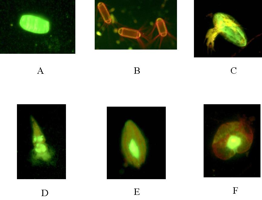
Figure 22. Selected photographs of microzooplankton stained with Acridine Orange that were
collected from the CTD casts on the NBP0202 Southern Ocean GLOBEC grid survey. A) Ciliate
Protozoan, Sta. 37 (40X,35 um length). B) Corethron sp. Diatoms, Sta.48 (20X, 65 um length).
C) Nauplius, Sta. 55 (40X, 50 um length). D) Tintinnid Ciliate, Sta. 37 (40X, 75 um length). E)
Ciliate Protozoan, Sta. 37 (40X, 62 um length). F) Dinoflagellate, Sta. 55 (40X,50um width).
5.2.1 Sound speed contrast measurements
To conduct this type of measurements, a specially designed Acoustic Properties Of Plankton (APOP) instrument was used during the cruise. The system was modified from the original version in order to make a series measurements in one cast. The basic idea of the APOP is to measure the time difference for acoustic waves or sounds traveling directly from one acoustic transducer (the transmitter) to another transducer (the receiver) with and without animals in the acoustic path. If sound travels faster in animal bodies than in water, the travel time with animals present in the acoustic path will be shorter and vice versa. The ratio of the sound speed in animals to that in water is called sound speed contrast or h, and is an important parameter used in describing acoustic scattering by weakly scattering objects such as krill.
A dual-chamber acoustic apparatus was used in the modified APOP, with one being a primary acoustic chamber holding animals and seawater, and the other as a secondary or a reference chamber holding just seawaer that can provide information reflecting relative sound speed changes at different depths. Each acoustic chamber contains two identical broadband transducers with a center frequency around 500 kHz and a bandwidth of about 300 kHz. The two chambers were mounted next to each other in a stainless steel bucket-shaped container.
5.2.2 Density contrast measurements
Similar to the sound speed contrast, the density contrast or g, is another important parameter used in describing acoustic scattering by weakly scattering objects. It is defined as the ratio of the density of the animals to that of the surrounding water. To measure the density, or density contrast of the krill on board the ship, a motion compensated dual-density method was used. The ship motion was compensated by using an additional electric balance. Two identical electric balances (Ohaus, AP210) were mounted on the same table next to each other, with one as a primary balance and the other as a reference balance. The latter had a calibration mass on its weighing platform throughout the measurement. Since both balances underwent the same accelerations, the fluctuations of the weight readings from the two balances were supposed to be simultaneous. The output digital readings from the two balances were received by a computer through the serial links (RS 232) and then the actual weight of the object being weighted on the primary balance could be inferred or calculated. The relative accuracy of this motion compensated weighing system was better than 0.02%.
5.3 Data Collection and Preliminary Results
The main focus of the material property measurements on krill during this cruise was to use live animals. To catch live krill as well as other live zooplankton, a 1 m diameter “Reeve” net was used, with a mesh size of 333 microns. The codend bucket of the Reeve net is much larger than those of MOCNESS, more than 4 times larger in volume. The krill that we caught were almost exclusively Euphausia superba. Other than krill, animals that were caught with Reeve net were copepods, mostly Calanus sp., amphipods (Parathemisto sp.), and diatoms (Table 6).
Table 6. Summary of Reeve Net Tows.
Cast # |
Date |
Station # |
Cast Depth (m) |
Catch |
1 |
4-15-2002 |
4 |
300 |
diatoms |
2 |
4-15-2002 |
7 |
100 |
a few adult and juvenile krill |
3 |
4-15-2002 |
7 |
100 |
more than 30 adult and 70 juvenile krill |
4 |
4-17-2002 |
11 |
400 |
diatoms |
5 |
4-18-2002 |
17 |
350 |
a few juvenile krill |
6 |
4-22-2002 |
29 |
165 |
a dozen adult and a number of juvenile krill |
7 |
4-22-2002 |
34 |
150 |
about 10 adult and a few juvenile krill |
8 |
4-25-2002 |
44 |
60 |
diatoms, copepods |
9 |
4-27-2002 |
50 |
360 |
more than 100 amphipods and thousands of copepods |
10 |
5-07-2002 |
82 |
435 |
lots of copepods, a few juvenile krill |
11 |
5-09-2002 |
41 |
375 |
copepods |
12 |
5-15-2002 |
|
100 |
more than 200 juvenile, sub-adult, and adult krill |
In addition to the animals we collected using the Reeve net, the group studying krill ecology and physiology lead by Dr. Kendra Daly on the L.M. Gould was willing to spare some of their live animals without interfering with their experiments. Through the two rendezvous with the Gould on April 23 and April 30, Kendra generously provided a large number of live krill (more than 200, E. superba and E. crystallorophias) and other zooplankton (mysids, amphipods, and copepods), as well as about 25 different sized fish (Pleuragramma) for use in the material properties experiments.
The APOP casts were all made from the surface to 205 m depth, except for the one on May 5 at station 77, where the water depth was only 180 m. The measurements were made at 20 m interval from 5 m to 205 m during both down and up casts. A total of 18 APOP casts were made. There were 16 casts with animals inside the APOP acoustic chambers (Table 7), including 10 with E. superba, two with E. crytallorophias, and two with copepods (Calanus). There were also two calibration casts made at the end of the cruise and two test casts made at the beginning of the cruise. The density contrast measurements were always conducted right after a sound speed measurement was made either on shipboard or during an APOP cast. The dual-density method was used throughout the cruise, except for one measurement of fish (Pleuragramma) where a displacement volume method was used instead.
There were total of 16 APOP casts, measuring the sound speed contrast of zooplankton, and corresponding density contrast measurements, as well as a number of shipboard measurements (Table 7).
One of the primary objectives of our project during this cruise was to study the temperature and pressure (depth) dependence of sound speed contrast of krill. The target species was E. superba and it was used in 10 out of 14 casts. The size range of the animals used in the casts varied from about 20 mm to 57 mm ( as measured from anterior to the eyeball to the tip of telson), which covered life stages from juvenile to sub-adult, and to the adult. We also made two APOP casts on another krill species, E. crystallorophias, whose minimum size was smaller than E. superba (Everson, 2000). The size distribution of the E. crystallorophias used in the two casts varied from 21 mm to 38 mm, with a mean size of 32 mm and a standard deviation of 3 mm, a much narrower distribution than that of E. superba.
There was no statistically significant depth dependence observed from the data sets involving E. superba, but there was a mild depth-dependence in sound speed contrast for E. crystallorophias, in which the sound speed contrasts were maximal at around 85 m and 105 m for the two casts, respectively.
For density contrast, all measurements were made in the ship lab. The mean density of 13 measurements made on krill E. superba was 1.025, with a standard deviation of 0.008. However, the density contrasts of E. crystallorophias from two measurements were 1.009 and 1.000, respectively, and were significantly smaller than the mean value of E. superba. Both the density and sound speed contrasts of the two krill species were relatively small compared with those of decapod shrimp (Palaemonetes vulgaris), whose sound speed and density contrasts are almost always greater than 1.04 (Chu et al., 2000a, b).
Although there were no statistically significant differences in measured sound speed and density contrasts between the freshly caught animals and those kept alive in aquariums for a longer time, there were slight size dependences observed from the data. Linear regressions showed that the density and sound speed contrasts had gradients of 5.485e-4 and 5.942e-4, respectively (Figure 23). This means that the difference of the target strength between a juvenile krill of size 27 mm and an adult krill of size 54 mm would be about 5 dB more than that resulting purely from size difference (6 dB in this case).
Figure 23. Sound speed and density contrasts of krill as a function
of the length of the krill. (a) Sound speed contrast as a function of
length. (b) Density contrast as a function of length.
Two APOP calibration casts were performed towards the end of the cruise on May 12 and May 15. The first one was conducted in the mouth of Marguerite Bay between Alexander Island and Adelaide Island and the second one was conducted in Crystal Sound. The objective of the calibration was to compare the differences in travel times between the two sets of transducer pairs that make up the APOP system. As noted above, one set of transducers is used for the primary acoustic chamber, which is filled with animals during a normal cast, and the other pair is in the reference chamber, which is kept empty during a cast. However, during the calibration casts, the compartments of both chambers were empty. The two calibrations casts gave the consistent results and will be incorporated in the later data processing.
Everson, I. (ed.), 2000. Krill, Biology, Ecology, and Fisheries. Blackwell Science Ltd., MA, USA.
Chu, D., P.H. Wiebe , and N. Copley, 2000a. “Inference of material properties of zooplankton from acoustic and resistivity measurements,” ICES J. Mar. Sci., 57:1128-1142.
Chu, D., P.H. Wiebe, T.K. Stanton, T.R. Hammar, K.W. Doherty, N.J. Copley, J. Zhang, D.B. Reeder, and M.C. Benfield, 2000b. "Measurements of the material properties of live marine organisms," Proceedings of the OCEANS 2000 MTS/IEEE International Symposium, Sept. 11-14, 2000, Providence, RI, Vol. 3, pp 1963-1967.
Table 7. Summary of Material Property Measurements on Zooplankton and Fish
Date |
Station |
Task |
Animal |
<L> (mm) |
g |
h |
4-16-2002 |
|
shipboard |
E. superba |
50.9 |
1.026 |
- |
4-17-2002 |
12 |
APOP cast 3 |
E. superba |
51.9 |
1.029 |
1.024 |
4-19-2002 |
21 |
APOP cast 4 |
E. superba |
26.9 |
1.007 |
1.018 |
4-23-2002 |
|
shipboard |
Pleuragramma antarticum |
60-70 |
1.018 |
1.017 |
4-23-2002 |
|
shipboard |
Pleuragramma antarticum |
69 |
1.007 |
1.013 |
4-23-2002 |
|
shipboard |
Eusirus sp. |
47.9 |
- |
1.096 |
4-23-2002 |
36 |
APOP cast 5 |
E. superba |
43.2 |
1.027 |
1.022 |
4-24-2002 |
|
shipboard |
Eusirus sp. |
47.9 |
1.051 |
1.038 |
4-24-2002 |
41 |
APOP cast 6 |
E. superba |
50.4 |
1.026 |
1.037 |
4-25-2002 |
|
shipboard |
Mysid arctomysis |
50.4 |
1.041 |
1.077 |
4-26-2002 |
|
shipboard |
Mysid arctomysis |
48.3 |
1.024 |
1.078 |
4-26-2002 |
|
shipboard |
E. superba |
36.6 |
1.027 |
1.048 |
4-27-2002 |
47 |
APOP cast 7 |
E. superba |
34.9 |
1.027 |
1.020 |
4-28-2002 |
|
shipboard |
Parathemisto sp. |
19.2 |
1.042 |
0.949 |
4-28-2002 |
54 |
APOP cast 8 |
E. superba |
52.7 |
1.026 |
1.040 |
4-29-2002 |
|
shipboard |
E. superba |
25.4 |
1.023 |
1.032 |
4-29-2002 |
55-56 |
APOP cast 9 |
E. crystallorophias |
32.3 |
1.009 |
1.025 |
5-01-2002 |
|
shipboard |
E. superba |
50.5 |
1.036 |
1.039 |
5-01-2002 |
62 |
APOP cast 10 |
E. superba |
50.5 |
1.036 |
1.044 |
5-02-2002 |
|
shipboard |
Calanus sp. |
4.1 |
0.995 |
0.959 |
5-02-2002 |
66 |
APOP cast 11 |
Calanus sp. |
4.1 |
0.995 |
0.949 |
5-03-2002 |
|
shipboard |
E. crystallorophias |
31.7 |
1.000 |
1.026 |
5-03-2002 |
71 |
APOP cast 12 |
E. crystallorophias |
31.7 |
1.000 |
1.030 |
5-04-2002 |
|
shipboard |
E. superba |
34.3 |
- |
1.021 |
5-04-2002 |
74 |
APOP cast 13 |
E. superba |
34.3 |
- |
1.020 |
5-05-2002 |
|
shipboard |
E. superba |
28.1 |
1.022 |
1.028 |
5-05-2002 |
77 |
APOP cast 14 |
E. superba |
28.1 |
1.022 |
1.024 |
5-07-2002 |
|
shipboard |
Calanus sp. |
3.2 |
0.996 |
1.012 |
5-07-2002 |
84 |
APOP cast 15 |
Calanus sp. |
3.2 |
0.996 |
1.023 |
5-15-2002 |
Crystal Sound |
shipboard |
E. superba |
27.1 |
1.017 |
1.034 |
5-15-2002 |
Crystal Sound |
APOP cast 17 |
E. superba |
27.1 |
1.017 |
1.030 |
6.0 Seabird and Crabeater Seal Distribution in the Marguerite Bay Area During NBP0202 (Christine Ribic [PI not present on cruise], Erik Chapman, Matthew Becker)
The association of seabirds with physical oceanographic features has had a long history. For example, seabirds have been found to be associated with temperature, water masses, currents, and the ice pack. Evidence for the association of seabirds with biological features has not been as strong. Veit (Veit, Silverman & Everson 1993), working during the breeding season at South Georgia, was not able to find a small-scale association of seabird distributions and krill patches. Only at a very large scale was there some evidence that there were more seabirds in the vicinity of krill patches than elsewhere. This may be due to the patchiness of the krill and the inability of seabirds to track these patches at small scales. Therefore, in the Antarctic system, seabirds may associate with physical features that have a higher probability of containing krill than associating with krill patches directly. The primary objective of the seabird project is to determine the distribution of seabirds in the Marguerite Bay area and to investigate their associations with physical and biological features. A second objective is to determine the foraging ecology of the seabirds in that area.
Because the SO GLOBEC cruises take place during the non-breeding season when birds will not be closely tied to nesting areas, we hypothesize that ability to detect enhanced food resources will be the driving factor determining seabird distributions.
We will be developing and testing competing models using existing knowledge of the marine system and Antarctic seabird biology. Models will be developed separately for each species or group of species based on their foraging ecology. We will be using seabird distribution and foraging ecology data that we collect along with data collected concurrently by physical and biological oceanographers to test these models.
Seabird distribution within the SO GLOBEC study area was investigated using daytime and nighttime (using night vision viewers) survey work, and foraging ecology of the Adelie Penguins was investigated through diet sampling. Nighttime surveys were designed to increase survey coverage of the study area when extended time on station and short days limited daylight survey time. During this cruise, Crabeater Seals (Lobodon carcinophagus) were observed in sufficient numbers to comment on their abundance throughout the study area. Diet sampling efforts are used to complement an Adelie Penguin (Pygoscelis adeliae) foraging ecology study being carried out by Dr. William F. Fraser on the RV Laurence M. Gould during the SO GLOBEC cruises. Surface tows, using a 1-m diameter ring-net, were carried out at CTD stations in order to sample prey available to seabirds throughout the study grid. A review of daytime surveys, diet sampling, and surface-tow effort and results are outlined separately below.
Strip transects were conducted simultaneously at 300 m and 600 m widths for birds. Surveys were conducted continuously while the ship was underway within the study area and when visibility was > 300 m. For strip transects, two observers continuously scanned a 90o area extending the transect distance (300 m and 600 m) to the side and forward along the transect line. Binoculars of 10X and 7X magnification were used to confirm species identifications. The 7X pair of binoculars also included a laser range finder. Ship following birds were noted at first occurrence in the survey transect. Ship followers will be down-weighted in the analyses because these individuals may have been attracted to the ship from habitats at a distance from the ship. For each sighting, the transect (300 m or 600 m), species, number of birds, behavior, flight direction, and any association with visible physical features, such as ice, were recorded. Distances were measured either by a range finder device as suggested by Heinneman or by the laser distance finder (when in the ice). Marine mammal sightings within the 600 m transect were also recorded. Primary ice-type and concentration within 800 m of the ship were also recorded and updated as they changed.
Surveys were conducted from an outside observation post located on the port bridge wing of the R/V NB Palmer. When it was not feasible to conduct surveys from this observation post, we surveyed from the inside port bridge wing.
Survey Locations: See Figure 24a.
Total Survey Time: 117 hours, 21 minutes
Distance Covered (km): 962.6
Boat Speed (knots): 4.9 (1.2 SD)
True Wind Speed (m/sec): 7.2 (3.1 SD)
Figure 24. a) Location of daytime surveys during NBP0202. The color of the survey
line corresponds to ice concentration during each transect. b) Open water species
(Southern Fulmar, Cape Petrel, Blue Petrel, Gray-headed Albatross, Wilson’s Storm
Petrel) abundance in the SO GLOBEC study area during NBP0202. Observation data
were interpolated spatially from mid-points of survey transects. They were classified
by standard deviations from the mean and darker shades are above the mean and lighter
shades below the mean. Ship-followers and birds attracted to the ship were down-weighted by 0.2
before being summarized for each survey transect. The color of the
survey line corresponds to ice concentration during each transect.
Ice conditions in the study area presented an interesting contrast between those of the first two SO GLOBEC cruises last year. During the first cruise, virtually the entire study area was ice-free, and during the second cruise it was mainly ice-covered. During this cruise, just the southern third of the study grid was covered in ice. The sea-ice appeared to be of two types; one-year-old ice separated by new ice types, and continuous new ice types. One-year-old ice covered 7 to 8/10ths of the ocean surface in George VI Sound. This ice extended to the northern tip of Alexander Island and then continued south, close to shore along the western shore of the island. Cold, still weather contributed to a large amount of new ice development during the cruise. By the time the ship reached the southern portion of the grid, combinations of new gray, new white, nilas, pancake and grease ice covered 8 to 10/10ths of the ocean surface. This new ice coverage was consistently observed on the 4 southern-most grid lines. New ice was also forming along the southwestern edge of Adelaide Island. Ice coverage during each survey is indicated in Figure 24a.
Overall, 2598 birds from 16 species were observed during the cruise. This is more birds and species than were observed during slightly less transect length during the previous two SO GLOBEC cruises (1771 birds from 13 species during SO GLOBEC I, and 895 birds from 6 species during SO GLOBEC II). Snow Petrels were the most abundant species, followed by Cape Petrels, Southern Fulmars and Antarctic Petrels. Overall observations during SO GLOBEC III are listed in Appendix 8.
Ice, as was observed during the first two SO GLOBEC cruises, appeared to be an important habitat variable that structures the seabird assemblage in the study area. In the northern, ice-free portion of the study area species known to forage in open-water habitat, such as Cape Petrel, Southern Fulmar, Albatross spp., Wilson’s Storm Petrel and Blue Petrel, were observed. A map interpolating open water species abundance from surveys across the study grid is presented in Figure 24b. Within the open water there appeared to be a concentration of open water species offshore and adjacent to the northern end of Adelaide Island, perhaps in association with the intrusion of Antarctic Circumpolar Deep Water observed by physical oceanographers during this cruise. Open water species also appeared to be concentrated near shore along the southwestern shore of Adelaide Island.
In the southern third of the study area where sea ice was present, Snow Petrels were the dominant species observed. A map interpolating Snow Petrel abundance from surveys across the study grid is presented in Figure 25a. These results were expected, as Snow Petrels are typically associated with ice cover, feeding at the interface between ice and open water. Within the sea-ice during this study, it appears that Snow Petrel abundance was highest in association with new ice at the interface between the developing pack ice and open water.
Figure 25. A) Snow Petrel abundance in the SO GLOBEC study area during
NBP0202. Observation data were interpolated spatially from mid-points of survey
transects. They were classified by standard deviations from the mean and darker
shades are above the mean and lighter shades below the mean. Ship-followers and
birds attracted to the ship were down-weighted by 0.2 before being summarized for
each survey transect. The color of the survey line corresponds to ice concentration
during each transect. B) Adelie Penguin abundance in the SO GLOBEC study area
during NBP0202. Observation data were interpolated spatially from mid-points of
survey transects. They were classified by standard deviations from the mean and
darker shades are above the mean and lighter shades below the mean. The color of
the survey line corresponds to ice concentration during each transect.
In the coming months, as data from other research groups on this cruise becomes available, we will be testing hypotheses that predict abundance of seabirds based on additional physical (including sea ice) and biological variables.
6.3.3.3 Adelie Penguin (Pygoscelis adeliae)
During the fall cruise last year, no Adelie Penguins were observed on the grid while during the winter cruise, Adelies were observed in small numbers throughout the pack in association with leads. During this cruise, Adelies were once again observed in pack ice, mainly in 7 to 8/10ths coverage where one-year-old ice as the primary ice-type in George VI Sound and along the westshore of Alexander Island. A map interpolating Adelie Penguin abundance from surveys across the study grid is presented in Figure 25b. Adelies were not observed in open water, or in association with ice-bergs and floes in any other area within the grid. Extrapolating the density of birds observed in the pack ice to the amount of area with one-year-old ice in the grid estimated that 17,000 Adelies were using this ice coverage in the study area. While this is a significant number of birds, it is a low number relative to the number of breeding birds in Marguerite Bay and the areas further north on the Antarctic Peninsula which number in the hundreds of thousands.
Off the grid, bird researchers on the L.M. Gould saw 80 birds on Avian Island on the southern shore of Adelaide Island. This island has 60,000 breeding pairs during the summer and these observations clearly indicate that the majority of the Adelies breeding here have moved elsewhere. However, observations made during diet sampling north of Adelaide Island in Crystal Sound, suggest that a significant number of birds may be using that area, rather than the region encompassed within the study grid. Groups of between 10 and 100 Adelies were observed porpoising in the water and resting on ice or land throughout the four hour period that we were in this area. The number of penguins in the immediate vicinity was estimated to be in the hundreds, possibly into the thousands. These observations are discussed in more detail in the general discussion section below.
6.3.3.4 Crabeater Seals (Lobodon carcinophagus)
The distribution of Crabeater Seals within the study grid are presented in Figure 26a. Crabeater Seals were concentrated north and along the western shore of Alexander Island and along the southwestern shore of Adelaide Island. The area near Alexander Island is the same region that Crabeater Seals were observed in high abundance during the fall cruise (SO GLOBEC I) last year. These seals may be associated with the concentration of krill observed by BIOMAPER-II in the deep canyons along the western shore of Adelaide during both of these cruises.
Figure 26. a) Crabeater Seal abundance in the SO GLOBEC study area during
NBP0202. Observation data were interpolated spatially from mid-points of
survey transects. They were classified by standard deviations from the mean and
darker shades are above the mean and lighter shades below the mean. The color
of the survey line corresponds to ice concentration during each transect. b)
Location of the Adelie diet sampling at the Barcroft Islands on May 15, 2002,
during NBP0202.
observed in high abundance during the fall cruise (SO GLOBEC I) last year. These seals may be associated with the concentration of krill observed by BIOMAPER-II in the deep canyons along the western shore of Adelaide during both of these cruises.
During SO GLOBEC cruises, we opportunistically diet sampled from the R/V N.B. Palmer according to protocols used by Dr. William R. Fraser. Dr. Fraser was diet sampling concurrently from the R/V L.M. Gould. We used the water off-loading technique in which birds are netted and their stomachs pumped using a small water pump. This technique is used extensively in seabird research in Antarctica [Antarctic Marine Ecosystem Research in the Ice Edge Zone (AMERIEZ), Antarctic Marine Living Resources Program (AMLR), Polar Oceans Research Group] and is preferable to methods that involve killing birds.
Fourteen Adelie Penguins were diet sampled from 5 distinct groups of birds in the Barcroft Islands (66 25' S; 67 10' W), south of Watkins Island and north of Adelaide Island (Figure 26b). Digested stomach contents that were not identifiable were separated from fresh contents. Fresh contents were further separated into krill, amphipod and fish components. Krill were identified to species and measured according to standard krill body-size measuring protocols.
After leaving the N.B. Palmer at 11:30 local time, birds were observed hauling out on small rock islands in the area beginning at 11:45. Adelies were captured, sampled and released throughout the afternoon until low light conditions concluded work at approximately 15:00. Body weights, sex, and stomach contents are reported in Appendix 9.
All birds sampled had fresh stomach contents that were easily identifiable, indicating that they had recently returned from foraging. Many of the birds had returned by 12:00 and were probably only foraging for 3 to 4 hours prior to sampling.
Overall, the Adelie diets were 63% Euphausia superba, 12% amphipods and 3% fish. Otoliths were collected from 5 of the 6 samples with fish parts. This is a distinct difference from Adelie stomach contents during the breeding season at Anvers Island that rarely contain components other than krill. The presence of relatively large amounts of amphipods is particularly unusual.
Body weights from the 8 male and 6 female penguins were high relative to summer weights and were an average of 4875 grams. These relatively heavy weights are indicators of excellent condition and could indicate preparation for a period of limited prey availability later in the winter.
Surface net tows were added to the research agenda this cruise in order to complement the physical and biological oceanographic data used for analysis of the seabird surveys. Near-surface resolution of prey species by BIOMAPER II is difficult, and thus net tows provided an additional means to help determine what types of prey seabirds could be feeding on at, or near, the ocean’s surface.
Surface net tows were conducted using a 1-m diameter (0.79 m2) ring net with 333 micron mesh. The net was lowered to a depth of approximately 60 m in the water column (while this is considerably deeper than any birds aside from penguins would be able to forage, it compensated for any vertical prey migrations that might be occurring) at an average rate of 30 m/min, then brought up at 10m/min. A general analysis of the sample composition was then made before preserving it in formalin. Tows were usually performed in the morning or evening periods in order to maximize the few hours of daylight available for surveying. Tows did not occur in heavy ice transects or at stations with MOCNESS tows.
6.3.5.3 Data Collected/Preliminary Results
A total of 22 samples were collected from 22 stations over the course of the grid (Figure 27). Results are summarized in Appendix 10. No extensive analysis of both the sample composition and correlations with seabird survey results will be able to be conducted prior to the conclusion of this cruise; however preliminary results were promising enough that surface net tows will be continued on SO GLOBEC IV.
Figure 27. Location of 22 1-m diameter ring net surface tows during NBP0202.
Blue circles indicate surface tows where no diatoms were not found and green
circles indicate where diatoms were found. These data will eventually be used
along with MOCNESS surface net data to look for spatial differences in species
composition and abundance of plankton at the surface. MOCNESS tow locations
are indicated by black triangles.
The most significant finding during this cruise may have been the large numbers of Adelie Penguins observed during diet sampling work in Crystal Sound. There are 17 breeding colonies with a total of 1600 pairs where the diet sampling was conducted in the Barcroft Islands. In addition, BIOMAPER-II, MOCNESS tows, and incidental observations from krill biologists on the L.M. Gould both last year and this year suggest that Crystal Sound has relatively large krill stocks at this time of year.
Adelies appear to have plenty of food and places to haul out in this area, and both the large numbers of birds and the large body sizes of the sampled birds suggest that this portion of the sound may represent a habitat optimum for the species at this time of year. Findings from Crabeater Seal research during SO GLOBEC also suggests that Crystal Sound may also have high Crabeater Seal abundance.
The Crystal Sound region provides an opportunity to further examine the physical and biological processes that are driving a system that appears to be attracting both seals and penguins. Because the interrelationship between physical and biological processes is the central focus of SO GLOBEC research, this area deserves attention in future research plans. Though it is possible that the same processes that existed during this time of year will have shifted with the development of sea-ice coverage later in the winter, it would be interesting to see if this area provides consistent habitat for Adelie Penguins throughout the winter survey and diet sampling work in this area is essential to assess the consistency with which penguins are utilizing Crystal Sound during the fall and winter months.
6.3.7 References
Veit, R.R., Silverman, E.D. & Everson, I. (1993) Aggregation patterns of pelagic predators and their principle prey, Antarctic Krill, near South Georgia. Journal of Animal Ecology, 62, 551-564.
6.3.8 Acknowledgments:
We would like to thank Captain Joe and all the ship’s mates for welcoming us on the bridge and putting up with the bird box on the port bridge wing during the cruise. We are particularly appreciative of the assistance of Gaelin Rosenwaks, Carin Ashjian, Ana Sirovic, Jenny White, and Steve Tarrant with the surface net tows. We would also like to thank Peter Wiebe and the other researchers on the ship for helping to schedule their work during the evenings so that we could survey for longer periods during the limited daylight available to us. Without that effort, our work would be seriously compromised.
7.0 International Whaling Commission Cetacean Visual Survey/span>
(Debra Glasgow)
Recently the International Whaling Commission (IWC) developed proposals for collaborative work in the Southern Ocean with the Commission for the Conservation of Antarctic Marine Living Resources (CCAMLR) and the International Global Ocean Ecosystem Dynamics (GLOBEC) program under the IWC Southern Ocean Whale Ecosystem Research (SOWER) program. This research program has the long term aim to “...define how spatial and temporal variability in the physical and biological environment influence cetacean species in order to determine those processes in the marine ecosystem which best predict long term changes in cetacean distribution, abundance, stock structure, extent and timing of migrations and fitness.”
This objective is being pursued through collaboration with GLOBEC and CCAMLR using a multidisciplinary ecosystem approach to data collection, analysis, and modeling. The IWC also recognizes that it lacks the data to determine baseline patterns of distribution (and the biological and physical processes responsible for such patterns) of baleen whales from which to judge the potential effects of climate change. Therefore, three further objectives have been defined by the Commission. They are: to characterise foraging behaviour and movements of individual baleen whales in relation to prey characteristics and physical environment, to relate distribution, abundance and biomass of baleen whales species to same for krill in a large area in a single season, and to monitor interannual variability in whale distribution and abundance in relation to physical environment and prey characteristics.
SO GLOBEC studies provide the ideal platform for such long term studies, where scientists from a range of disciplines can conduct intensive focused studies, within the framework of long term data synthesis and planning. Given the shared objectives among the IWC, GLOBEC and CCAMLR, the IWC has determined that the most effective means of investigating these ecological issues is to focus a considerable body of cetacean research within the framework provided by these programs (taken from D.Thiele).
The first of the 'Predator Science Questions' in SO GLOBEC has been formulated as: How does winter distribution and foraging ecology of top predators relate to the distribution and characteristics of the physical environment and prey (krill) (taken from J.A. van Franeker).
Standard IWC methodology for multi-disciplinary studies is being used throughout all GLOBEC collaborative cruises. This involves experienced cetacean researchers conducting line transect sighting surveys throughout daylight hours in acceptable weather conditions. Data are recorded on a laptop based tracking program (Wincruz), and photo and video records are also obtained for species identification, group size verification, feeding (and other behavior), ice habitat and individual identification (taken from D.Thiele).
During this cruise, observations were made from the ice tower by a single observer (Debra Glasgow). When conditions permitted, the observer was outside along the cat- walk of the ice tower, otherwise observations were made from the inside. Effort was focused 45o to port and starboard of the bow ahead of the vessel, while also scanning to cover the full 180o ahead of the vessel. In ice, the method was adjusted to include searching behind in the vessel's wake as well, in order that cetaceans and seals hidden by ice would be detected more readily. The observer used a combination of eye and binocular searching (7x50 Fujinon). Effort would commence when the following conditions allowed: appropriate daylight, winds less than 20 knots or Beaufort sea state less than 5-6, visibility greater than 1 nautical mile (measured by the distance a minke whale blow could be seen with the naked eye as judged by the observer) and the ship actually steaming. An Incidental watch was kept in borderline conditions or in variable visibility such as fog and snow squalls. Subjective weather data was recorded to keep track of the changing conditions e.g. Beaufort sea state, cloud cover, glare, ice, sight ability etc.
Sightings were recorded on a laptop based Wincruz Antarctic program which also logged GPS position, course, ship speed, and a suite of other environmental and sightings conditions automatically. Visual observations were made both during the station-transect portion of the trip, as well as during transit. When possible, photographic and/or video documentation was made of each sighting for later use in individual identification, species confirmation, and habitat description.
Generally, sighting conditions were poor, particularly during the first half of the cruise. The appropriate combination of environmental and ship conditions were not conducive to good sighting conditions. Yet 183 hours and 34 minutes of “On Effort” and “Incidental” survey effort were made during the entire cruise.
A total of 54 cetacean sightings of 112 animals were made (Appendix 12, Figure 28). These include 21 sightings of 49 humpback whales, Megaptera novaengliae and 10 sightings of 25 'like' humpback whales (Figure 29A); 5 sightings of 7 minke whales, Baleanoptera acutorostrata and 3 sightings of 3 'like' minke (Figure 29B); 2 sightings of 7 killer whales, Orcinus orca (Figure 29C); 1 sighting of 1 Commerson's dolphin, Cephalorhynchus commersonii; 2 sightings of 4 unidentified dolphins; 8 sightings of 12 various unidentified whales (Figure 29D); 1 sighting of a 'like' blue whale, Baleanoptera musculus (Figure 29E).
Figure 28. Distribution of Cetacean sightings on NBP0202 (See Appendix 12 for more
details).
Figure 29. Distribution of selected whales species sightings
Photo identification photos/video were obtained from at least six groups of humpbacks (WOS#10,13,19,20,50,52) and digital images of habitat, sea and ice conditions were taken. On 17 May 2002, as we steamed through Gerlache Strait, some ship time was made available to obtain ID photographs. One group of 3 humpback whales (WOS#52) was extremely cooperative - swimming to the ship and remaining within 10 to 30 metres of the vessel for over half an hour, even following the ship briefly as we left, allowing good images to be taken (Figure 30).
Figure 30. Digital images of whales taken on NBP0202. A) Humpback dorsal fins #1
& #2 - WOS#52, 17 May 2002 (Photo by Kristin Cobb). B) Dorsal fin of Humpback
whale #3 - WOS#52, 17 May 2002 (Photo by K. Cobb). C) Humpback whale fluke -
WOS#52, 17 May 2002 (Photo by Ana Sirovic). D) Dorsal fin of Humpback whale -
WOS #19, 25 April (Photo by A. Sirovic) E) Humpback dorsal fin #1 & head -
WOS#52, 17 May 2002 (Photo by K. Cobb). F) Humpback whale fluke - 25 April
2002 (Photo by A. Sirovic). G) Humpback whales off the bow (64 32.59' S; 62 30.33'
W) - WOS#52, 17 May 2002 at 1251 (Photo by A. Sirovic). H) Humpback whales -
white flank markings whales #1 & #3 - WOS#52, 17 May 2002 (Photo by A. Sirovic).
On 17 April 2002 a 'like' blue whale body was sighted underwater to port, swimming away from the vessel and Ana Sirovic was recording good blue whale sound from a sonobuoy at that time.
7.4 Preliminary Findings/Discussion
Sightings data from this cruise show mainly humpback (Megaptera baleanoptera), minke (Baleanoptera acutorostrata), and killer whales (Orcinus orca) present in the study region in the austral fall and beginning of this winter.
Correlation of cetacean distributions with concurrent hydrographic distributions show whales associated with: 1) the southern boundary of the Antarctic Circumpolar Current, 2) the frontal boundary between intrusions of warm Upper Circumpolar Deep Water and continental shelf water, and 3) the frontal boundary between inner shelf coastal current and continental shelf waters (E.Hoffman pers. Comm).
Humpback sightings were particularly numerous along the mid shelf area just outside Marguerite Bay, along the continental shelf and near the frontal boundary formed as the coastal current exits the Bay. There was also a group of humpbacks near the ice edge off Alexander Island associated with a patch of krill recorded by the BIOMAPER-II team. Minke sightings were more widespread, but seemed to be associated closer to the ice edge and to the coastal frontal boundaries. Killer whales were seen within the ice edge on both occasions in areas where large numbers of seals were recorded.
The correspondence between the cetacean sightings and hydrographic features suggests that the austral fall/winter distribution of cetaceans along the west Antarctic Peninsula is not random, but rather is determined by the structure of the physical environment, which in turn determines prey distribution. Continued analyses and collection of sightings data in conjunction with concurrent prey and hydrographic distributions will allow determination of the causal relationships underlying austral fall/winter cetacean distributions in the Antarctic Peninsular region (D.Thiele).
Thanks must go to the Captain and crew of the N. B. Palmer, the cruise leader - Peter Wiebe, and to the scientists and support staff on board for their expert help and friendship. Thanks also to the bird observers Erik Chapman and Matt Becker for extra help in gathering data and to Suzanne O'Hara for mapping work.
Related US SO GLOBEC reports for previous cruises 1,2,3 – and particularly NBP01-03 1st cruise (survey cruise) – US Southern Ocean GLOBEC Report No.2
Friedlander A.S., Thiele D., Hoffman E., MacDonald M.., Moore S., Pirzl R. A preliminary analysis of baleen whale distribution around the western Antarctic Peninsula in the Austral fall and winter.
Website for IWC cetacean summaries by cruise, cruise reports, and technical US SO GLOBEC reports
http://www1.npm.ac.uk/globec/ this site provides a direct link to the CCPO site by clicking on SO GLOBEC
8.0 Marine Mammals Passive Acoustics (Ana Sirovic)
8.1 Introduction
The primary goal of this project is to determine the minimum population estimates, distribution and seasonality of mysticete whales within the West Antarctic Peninsula region. These data will be integrated with the rest of the SO GLOBEC data set to improve the understanding of krill ecology in the area. Because the vocalizations of most baleen whales are species specific and easily recognizable, passive acoustic techniques can be used to determine long-term, seasonal presence of a species in the area. The species of interest are blue (Balaenoptera musculus), fin (B. physalus), humpback (Megaptera novaeangliae) and Antarctic minke (B. bonaerensis) whales. Southern right whale (Eubalaena australis), sperm whale (Physeter macrocephalus - odontocete) calls may also be detected, but are expected less frequently. The key component of this study is a series of 8 acoustic recording packages (ARPs) that were recovered and redeployed during the LMG02-01A cruise (Feb 5 to Mar 3, 2002). They are bottom mounted and have a hydrophone component floating 5 m above the mooring. Each ARP yielded approximately 28 GB of data after the initial 11 months of deployment and they are currently recording for another 12 months.
During this cruise, sonobuoys were deployed opportunistically to supplement the information obtained from the visual observations, as well as the ARP data. Sonobuoys are expendable underwater listening devices. Four main components of a sonobuoy are a float, radio transmitter, saltwater battery, and hydrophone. The hydrophone is an underwater sensor that converts the sound pressure waves into electrical voltages that get amplified and sent up a wire (hydrophone depth can be set to 90, 400, or 1000 feet) to the radio transmitter that is housed in the surface float. The radio signal is picked up by an antenna and a radio receiver on the ship, then reviewed and simultaneously recorded onto a digital audio tape (DAT). A sonobuoy can transmit for a maximum of 8 h before scuttling and sinking.
Two types of sonobuoys were deployed: omnidirectional (57B) and difar (53B). Omnidirectional sonobuoys have hydrophones that can register signals up to 20 kHz, but they cannot determine the location of the sound source. DiFAR (DIrectional Fixing And Ranging) sonobuoys also have an omnidirectional hydrophone for recording sound, but it is limited to frequencies lower than 4.5 kHz. However, DiFARs also have 2 pairs of direction sensors, which along with an internal compass can determine the exact bearing of the sound relative to the sonobuoy. With 3 or more sonobuoys in the water, it is thus possible to determine the location of the sound source.
The Yagi directional antenna was used primarily during the cruise. The maximum range for the radio transmission during this cruise was 16 nm, but the range seemed highly dependent on weather conditions. The Sinclair omnidirectional antenna was also available throughout the cruise, but the maximum range obtained by that antenna was less than 3 nm and it was, therefore, not used very often. The problem with having to use the Yagi all the time was that sonobuoys could be heard only while steaming in a straight line. Once we were at a station and the ship started turning, signal was quickly lost.
There were several reasons for sonobuoy deployments. Firstly, they provide recordings that can be compared to the ARP data. This will provide a calibration on content as well as detection ranges. Secondly, they are a means of getting recordings outside of the seafloor array range. Lastly, they are a good complement to the visual observations and can help in positive identification of species when visual cues are not.
Sonobuoys were deployed both when whales were visually detected and randomly throughout the cruise. A total of 62 sonobuoys were deployed: 57 omnidirectional and 5 DiFARs. Only 4 omni sonobuoys failed upon deployment, which is a satisfactory performance. Locations of all the deployments as well as a preliminary summary of the sonobuoys on which calls were heard can be seen in the complete (Figure 31) and close-up (Figure 32) maps of the study area. Further analysis of the recordings is needed to double check for calls that were possibly not detected during the preliminary review. The locations and times of all the deployments are given in the cruise Event Log.
Figure 31. Sonobuoy deployment locations with species heard on the sonobuoy marked. Calling
whales can be heard at large distances from the sonobuoy so a detected call does not necessarily
indicate immediate vicinity of whales.
Figure 32. Close-up of the study area with the sonobuoy deployment locations marked. If any calls
were heard on the sonobuoy, it is marked with the appropriate symbol.
Species heard on the highest number of sonobuoys were blue whales. All 19 buoys that blues were heard on, however, were deployed in the northern part of the grid, either on the outer shelf or off the shelf break (where the loudest recording was obtained). No blues were heard on any of the sonobuoys deployed while steaming under ice or in Marguerite Bay. Blue whales were also heard on a couple of the sonobuoys deployed while steaming towards the grid stations at the beginning of the cruise.
Humpbacks were the second most commonly heard species; their calls were heard on 17 sonobuoys. Most of the calls resembled the song phrases that were recorded last year during GLOBEC I. The distribution of calling humpbacks, however, was quite different from the one observed during the last fall’s cruise. They were heard on sonobuoys deployed while steaming along transect lines 4 and 5 on and off the shelf, and again in the same area as we were steaming north after the end of grid work. No humpbacks were heard in Laubeuf fjord, though, where a lot of them were recorded last year. Also, instead of being concentrated around northern tip of Alexander Island like they were last year, this year the humpbacks were more spread out along the shelf due west from the northern edge of Alexander. Humpbacks were heard on one sonobuoy deployed in Crystal Sound and on both of the sonobuoys deployed in the Gerlache Strait during the steam back north. A possible fin whale was heard on the northernmost deployed sonobuoy in the Drake Passage. No minke whale calls were heard in the
preliminary analysis. Unidentified odontocete whistles were recorded twice, and clicks preceded those whistles on one occasion. Both of the recordings were obtained while ice was present. An unidentified seal was also heard on a sonobuoy deployed while we were steaming north from the end of the grid.9.0 Fish Otolith Collections (Julian Ashford, ODU)
Field sampling was undertaken for a pilot study to examine the relationship between water mass and the chemical signature laid down in the calcium carbonate matrix of the otoliths of fish. If signatures can be discriminated spatially, they can theoretically be used as an internal tag to trace fish movement in space and, using the chronology laid down concurrently in the otoliths, through time and by age. The tags can then be used to estimate age-based population migration rates and site fidelity. As the uptake of trace elements is primarily from the surrounding water mass, the first-order variables influencing the chemical signature are likely to be hydrographic. The current cruise represents the first opportunity in the Antarctic to use linked carbonate chemistry and hydrographic data sets to examine water mass effects on the chemical signature and, once this is better understood, potentially further elucidate the role played by ocean dynamics in fish movement and life history.
Sampling events on board the RVIB Nathaniel B. Palmer, including MOCNESS, Reeve net, and surface net tows, were monitored for fish by-catch. Data taken during the CTD cast at the same station were used to identify water mass. Sampling of fish was considered conditioned on water mass, with spatially-based sampling units taken from a fixed frame composing the cruise grid, using a stratified hierarchical random sampling method. A limited number of samples were taken, mostly in the northern part of the grid, including species from the genera Bathylagus, Protomyctophum, Gymnoscopelus, and Electrona. These will be supplemented by collections made during the same time period on board the R/V Lawrence M. Gould, including Pleuragramma antarcticum.
Using the Laser-ICPMS facility funded by NSF at Old Dominion, comparisons will be made between the otolith signatures from samples taken from different water masses. Further comparisons are also planned between years using available samples and hydrographic data from the 2001 GLOBEC cruises, to examine the stability of the signature in time.
10.0 Science Writer Report (Kristin Cobb UCSC/NSF)
The job of the National Science Foundation (NSF) science writer was to report on the scientific activities of the third U.S. SO GLOBEC cruise. The broader goals were to make science accessible and engaging to a general audience and to describe the challenges and rewards of working on an Antarctic research vessel. Dispatches and photographs are located at http://www.nsf.gov/od/lpa/news/02/pr0236_dispatches.htm.
The first story explained the overall goals of research to be conducted on the RVIB Nathaniel B. Palmer and the R/V Laurence M. Gould. The subsequent dispatches chronicled the trip, while each focusing on a different major scientific group. Scientific groups covered in-depth included: Conductivity, Temperature, Depth (CTD), BIo-Optical Multi-frequency Acoustical and Physical Environmental Recorder (BIOMAPER-II), Acoustical Properties of zooPlankton (APOP), seabird survey and field work, and marine mammal survey and field work. In addition, a profile of the Palmer's captain was written. The stories focused on people as much as science, and attempts were made to include the voices of scientists from the Laurence M. Gould, as well as of the science support staff and of the crew aboard the Palmer.
11.0 Seabeam bathymetry of region and Mooring surveys (Suzanne O’Hara)
The multibeam bathymetric data for NBP0202 - GLOBEC III was collected with a SeaBeam 2112 system. This instrument generates 120 bathymetric and 2,000 sidescan across swath values for each ping. The total width of the data swath is 120 degrees, or about three times the depth of the water that is being surveyed. This system has been in use on the N.B. Palmer since 1994 and it will be removed from the ship after this cruise.
The SeaBeam was run continuously while the ship was underway and after the vessel was over 200 miles away from Chile and Argentina. A total of 806 hourly multibeam files were collected between April 12, 2002 (year day 102) and May 19, 2002 (year day 139) over approximately 3,536 miles of ship track. All of these files were ping edited by the science party to remove errors from the raw data. The cleaned data files were merged with multibeam data collected during other cruises to generate gridded data files and survey plots. Fifty three separate survey areas were identified, gridded and plotted. A small scale plot of the main survey area is included with this report (Figure 33).
Figure 33. A composite view of the Southern Ocean GLOBEC bathymetry based
on the SeaBeam surveys done in the area that are publically available.
Science Party (Name, Institution)
Zooplankton and Krill Survey (BIOMAPER-II, 1-m2 MOCNESS, ROV)
Wiebe, Peter Woods Hole Oceanographic Institution
Ashjian, Carin Woods Hole Oceanographic Institution
Dennett, Mark Woods Hole Oceanographic Institution
Alatalo, Philip Woods Hole Oceanographic Institution
Girard, Andy Woods Hole Oceanographic Institution
Kukulya, Amy Woods Hole Oceanographic Institution
Martin, Peter Oregon State University
Rosenwaks, Gaelin Woods Hole Oceanographic Institution
Taisey, Phillip Northeastern University
Zooplankton Material Properties
Chu, Dezang Woods Hole Oceanographic Institution
Riener, Karen
CTD/ADCP
Klinck, John Old Dominion University
Ashford, Julian Old Dominion Universty
Sepulveda, Hector Andres Old Dominion Universty (Chile)
Boyer, Timothy National Oceanographic Data Center
Mackay, Chris RGL Consulting LTD, Canada
Nutrients
Masserini, Rob University of South Florida
Serebrennikova, Yulia Univeristy of South Florida
Productivity Measurements
Kozlowski, Wendy Scripps Institution of Oceanography
Aller, Kristy Scripps Institution of Oceanography
Seabird Survey/Ecology
Chapman, Erik University of Wisconsin
Becker, Mathew
Whale Survey/Active Counting
Glasgow, Deb IWC (New Zealand)
Whale Survey/Passive Listening
Sirovic, Ana Scripps Institution of Oceanography
Science Writer
Cobb, Kristin NSF/University of California, Santa Cruz
Raytheon Technical Support
Doyle, Alice Marine Project Coordinator
Alesandrini, Stian Marine Technician
Tarrent, Steve Marine Technician
White, Jennifer Marine Technician
Bliss, Kevin Information Technology
O’Hara, Suzanne Information Technology
Martellero, Helena Information Technology
Blackman, Sheldon Electronics Technician
Lariviere, Romeo Electronics Technician
Ship’s Officers and Crew
Borkowski, Joe Master
Wisner, Richard Chief Mate
Repin, Vladimir 2nd Mate
Higdon, John 3rd Mate
Pagtalunan, Rachelle 3rd Mate
Pierce, Johnny Chief Engineer
Ambrocio, Rogelio 1st Engineer
Sykas, Peter 2nd Engineer
Zipperer, Bryan 3rd Engineer
Hanna, George 3rd Engineer
Rogando, Rolly Oiler
Pagdanganan, Rogelio Oiler
Delacruz, Fredor Oiler
Villanueva, Sam A.B.
Sandoval, Lorenzo A.B.
Tamayo, Ric A.B.
Carpio, Ronnie A.B.
Aaron, Bienvenido A.B.
Monje, Alejandra A.B.
Silverio, Nestor O.S
Wisner, Theresa O.S.
Cardenas, Yessica O.S.
Appendix 2. Summary of CTD casts
Appendix 3. Summary of water samples
Appendix 4. Summary of salinity measurements
Appendix 5. Summary of oxygen titrations
Appendix 6. Summary of expendable probes
Appendix 7. Video and Lugol's Samples Taken on NBP0202
Appendix 8. Summary of sightings
Appendix 9. Results from analysis of fourteen diet samples of Adelie Penguins
Appendix 10. 1-m Ring Net Tow Information.
Appendix 11. BIOMAPER-II Tape Log.
Appendix 12. Cetacean Sightings NBP0202 9 April to 21 May 2002